IJCNC 08

ON THE PERFORMANCE OF INTRUSION DETECTION SYSTEMS WITH HIDDEN MULTILAYER NEURAL NETWORK USING DSD TRAINING

Trong Thua Huynh, Hoang Thanh Nguyen
Posts and Telecommunications Institute of Technology, Ho Chi Minh City, Vietnam

---

ABSTRACT

---

Deep learning applications, especially multilayer neural network models, result in network intrusion detection with high accuracy. This study proposes a model that combines a multilayer neural network with
Dense Sparse Dense (DSD) multi-stage training to simultaneously improve the criteria related to the performance of intrusion detection systems on a comprehensive dataset UNSW-NB15. We conduct experiments on many neural network models such as Recurrent Neural Network (RNN), Long-Short Term Memory (LSTM), Gated Recurrent Unit (GRU), etc. to evaluate the combined efficiency with each model through many criteria such as accuracy, detection rate, false alarm rate, precision, and F1-Score. 

KEYWORDS

---

UNSW-NB15, deep learning, IDS, neural network.

1. INTRODUCTION

---

An Intrusion Detection System (IDS) is a network traffic monitoring system, capable of recognizing suspicious activities or unauthorized intrusions on the network during an attack, thereby providing identifiable information and giving warnings to the system and administrator. The development of malware poses an important challenge to the design of IDS. Malware attacks have become more sophisticated and challenging. Malware creators can use a variety of techniques to conceal their behavior and prevent IDS from being detected, so they can easily steal important data and disrupt the business operations of numerous individuals and organizations.

IDS works in three main ways: Signature-based, Anomaly-based, and Stateful Protocol Analysis. Signature-based IDS compares signatures of the observed object with those of known threats. Anomaly-based IDS compares definitions of normal activities and the observed object to identify deviations and generate alarms. Stateful Protocol Analysis IDS compares predetermined profiles of the behavior of each protocol that is considered normal with the observed object to determine deviations. Except for the Signature-based method, the two other methods need to be learned to recognize anomalies. Therefore, over the past few decades, machine learning has been used to improve intrusion detection.

The effectiveness of IDSs is evaluated based on their performance in identifying attacks. This requires a comprehensive dataset including both normal and anomalous behaviors. Previous datasets such as KDDCUP99 [1] and NSL-KDD [2] have been widely applied to evaluate the performance of IDSs. Although the performance of these datasets has been acknowledged in many previous studies, the evaluation of IDS using these datasets does not reflect the actual output performance due to several reasons. The first reason is that the KDDCUP99 dataset contains a large number of redundant records in the training set. Redundant records affect the results of biases in intrusion detection for frequent records. Second, the fact that many records are missing is also a factor that changes the nature of the data. Third, the NSL-KDD dataset is an improved version of KDDCUP99, which solves some problems such as data imbalance between normal and abnormal records as well as missing values [3]. However, this dataset is not a comprehensive representation of the actual modern attack environment. The standard dataset UNSW-NB15 [4] was created to address the limitations of the previous datasets, especially, it is regularly updated with new data features and attacks.

There have been many machine learning methods and neural network models applied to network intrusion detection such as RNN, LSTM, GRU. Choosing the right model for the UNSW-NB15 dataset to improve the evaluation results is also a matter of concern [5]. In addition, one of the recent studies to improve training quality is that the DSD (Dense Sparse Dense) training model [6] has been applied effectively to some image processing and voice recognition problems. In this study, we focus on evaluating the efficiency of network intrusion detection based on deep neural network models such as RNN, LSTM, GRU by proposing a model that combines the DSD training method into each of these neural network models to improve the performance of network intrusion detection systems.

The remainder of the paper is organized as follows. In section 2, we present the related work. Section 3 describes the proposed hybrid model. Sections 4 and 5 present the experiment, result, and evaluation of the proposed models. Finally, concluding remarks are given in section 6. 

2. RELATED WORK

---

2.1. Deep Neural Network

The neural network is a technique created to simulate the human brain for pattern recognition and are used in a variety of learning tasks. Generally, it consists of three layers, one for input, one for output, and at least one hidden layer between them. The input goes from the input layer through the hidden layers, to the output layer through a set of neuronal nodes in each layer, whether it is a linear or non-linear relationship. DNN shows that there is more than one hidden layer in a neural network. It is widely used in supervised and unsupervised learning, as well as for classification and clustering. In a few recent studies, DNN is widely used in detecting network intrusions [7] and web phishing [8].

In this model, a group of neurons is passed to the hidden layers as input data. These neurons are connected by the weight factor, which represents the importance of the input value. The more valuable neurons, the greater the impact on the next layer of neurons. Many types of Artificial Neural Networks have been developed, the first and simplest Neural Network widely used is the Feed-Forward Neural Network. In this type of network, information is transmitted in parallel from the input layer directly through the hidden layers and then into the output layer without loops.

2.2. Recurrent Neural Network (RNN)

RNN [9] is an extension of a straightforward neural network, designed to recognize patterns in data series. This network is regressive because it performs the same task for every element of the sequence with the output depending on previous computations. [10].

RNN can be viewed as a way to share weights over time, as illustrated in Figure 1. The following equations (1) and (2) are used to compute the state ht and the hidden output Ot in terms of the RNN:

Where σ and 𝜏 are sigmoid and softmax activation functions, respectively, xt is an input vector at time t, ht is a hidden state vector at time t, Wi is an input weight matrix, U is a weight matrix between hidden layers, Wo is the output weight matrix and bt is the bias coefficient.

Figure 1. Simple RNN architecture

The RNN model has a major drawback, at each time in the training process, similar weights are used to compute the O_t output, which causes the output to be incorrect. Long Short-Term Memory (LSTM) and Gated Recurrent Unit (GRU) models have been proposed to solve this problem.

2.3. Long Short-Term Memory (LSTM)

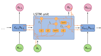
The Long Short Term Memory (LSTM) network [9] is a variant of the recurrent neural network proposed as one of the machine learning techniques to solve many sequential data problems. LSTM helps maintain errors that can propagate back layers over time. LSTM is used to increase the accuracy of the output, as well as to make the RNN more useful for long-term memory tasks. The LSTM architecture, as illustrated in Figure 2, consists of four main components; input port (i), forget port (f), output port (o), and memory cell (c).

Figure 2. The core architecture of the LSTM block [9

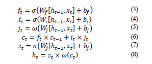
The LSTM block makes decisions about whether to store, read, and write through open or closed ports,  and each block of memory corresponds to a specific time. The communication ports are based on a set of weights. Some weights, like input and hidden states, are adjusted during the learning process. Equations from (3) to (8) are used to represent the relationship between input and output at time t in each LSTM block.

Where σ and w are the activation functions sigmoid and tanh, respectively, x_t is an input vector at time t, h_t is the output vector at time t, W and b are the weight matrix and bias coefficient, respectively. f_t is a forget function used to filter out unnecessary information, i_t and j_t are used to insert new information into memory cells, z_t outputs relevant information.

2.4. Gated Recurrent Unit (GRU)

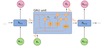
GRU is a variant of LSTM introduced by K.Cho [10]. Basically, The GRU is an LSTM with no output ports, so it writes all the content from memory to the larger network at a time. However, it is refined using an updated gate that is added to the GRU block. The updated port is a combination of an input port and a forget port. The GRU model is proposed to simplify the architecture of the LSTM model. The structure of the GRU is shown in Figure 3. Equations (9) to (12) show the relationship between the input and the predicted outcome.

Figure 3. The core architecture of the GRU block [9]

Where the feature space (input) is represented by x and the prediction is represented by o_t, v_t is the updated function. W is the weight optimized during the training process. σ and w are sigmoid and tanh activation functions respectively to keep the information passing through the GRU within a specific range.

2.5. Dense Sparse Dense (DSD)

Complex multi-layer neural models give good results and can obtain highly nonlinear relationships between feature data and output. The disadvantage of these large models is that they are prone to noise in the training dataset. This leads to overfitting [11] and high variance [12]. However, if the model is reduced to a less complex form, the machine learning system may miss the relevant relationships between the features and the output, leading to the problem of under-fitting [11] and high bias [13]. This is a very challenging problem because bias and variance are difficult to optimize at the same time.

By pruning and re-dense the network, the DSD training model changes the optimization process and improves the optimization performance with significant results. Some of the factors that make the DSD training model effective are:

• Saddle point: DSD overcomes saddle points by trimming and thickening the model.
• Significantly better minima: DSD reduced the loss and error on both the training set and the validation on ImageNet.
• Frequent and Sparse Training: Both sparse training and DSD ultimately reduce the variance and lead to lower errors.
• Strong Re-initialization: DSD allows to optimize second chances during training to restart using a robust sparse training solution.

In the study [6], Song and colleagues introduced DSD, a “dense – sparse – dense” training model by selecting connections to discard and recover others later. The authors tested their DSD model with GoogLeNet, VGGNet, and ResNet on the ImageNet dataset, NeuralTalk BLEU on the Flickr-8K dataset, and DeepSpeech-1&2 on the WSJ’93 dataset. Experimental results show that the DSD training model has brought significant efficiency on image processing and voice recognition datasets applied on deep neural networks.

3. Hybrid Neural Network Model

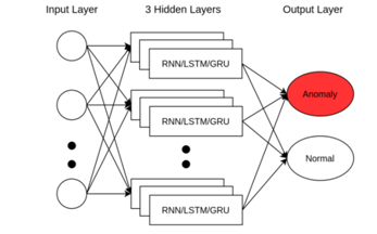
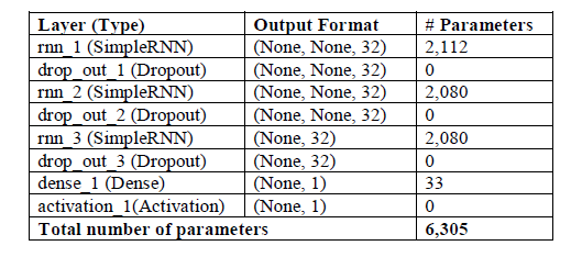
Realizing that recurrent neural networks (RNN/LSTM/GRU) can effectively learn to generate highly nonlinear relationships between input and output features, this study proposes a hybridmodel combining RNN/LSTM/GRU with a 3-stage DSD training scheme to improve network intrusion detection efficiency. We set the number of neurons of all hidden layers to 32. The proposed model includes:

Figure 4. Simple RNN/LSTM/GRU architecture with layers 3 hidden

• The simple 3 hidden layers RNN/LSTM/GRU neural network is shown in Figure 4;
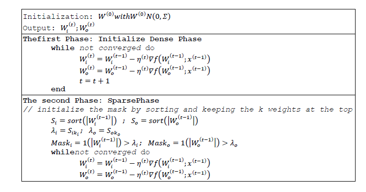
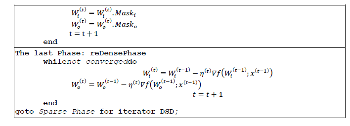
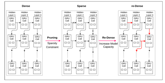
• The hybrid training model DSD-3hRNN/DSD-3hLSTM/DSD-3hGRU uses a three-stage process: dense (Dense – D), sparse (Sparse – S), re-dense (reDense – D) is applied on the simple neural network model with 3 hidden layers (3h). The stages are illustrated in Figure 5 (DSD-3hRNN), Figure 6 (DSD-3hLSTM), and Figure 7 (DSD-3hGRU).

The proposed model contains three hidden layers. Each layer is fully connected to the next layer in the network, where ReLU function is used in hidden layers and sigmoid function is used in the output layer for binary classification while the softmax function is used in the output layer for multiclass classification.

3.1. Determining the number of hidden layers

Problems requiring more than two hidden layers are unusual for deep learning. Two or fewer layers are usually sufficient with simple datasets. However, with complex datasets, additional layers can be useful. The following table summarizes the capabilities of some popular layered architectures. We can clarify this as follows:

• If the number of hidden layers is one, the result can approximate any function that contains a continuous mapping from one finite space to another.
• If the number of hidden layers is two, the result can represent an arbitrary decision boundary to arbitrary accuracy with rational activation functions and can approximate any smooth mapping to any accuracy.
• If the number of hidden layers is more than two, additional layers can learn complex representations.

Besides, we tried to train the model with more than 3 hidden layers, the result is not only similar to the 3-hidden layer model but also takes more time. Therefore, we decided to choose a 3-hidden layer model for this dataset.

3.2. Determining the number of neurons in hidden layers

Using too few neurons in hidden layers will lead to under-fitting. Using too many neurons in hidden layers can lead to over-fitting problems. To select the number of neurons per hidden layer, we use some rules as follows:

• The number of neurons in the hidden layer is between the size of the input layer and the size of the output layer.
• The number of neurons in the hidden layer is 2/3 the size of the input layer, plus the size of the output layer.

The number of neurons in the hidden layer is less than twice the size of the input layer

“

Figure 5. Hybrid DSD-3hRNN model

Table 1. Configuration of the proposed 3 hidden-layer DSD-3hRNN model

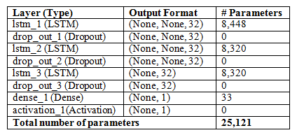
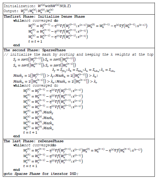
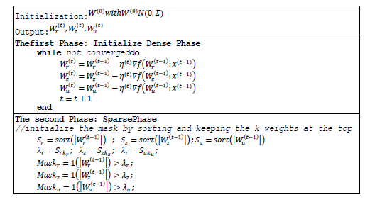
The model of 3 hidden layers with LSTM using DSD training is shown in Figure 6. The recommended configuration of the DSD-3hLSTM model is described in Table 2. The detailed training procedure is described in Algorithm 2.

Table 2. Configuration of the proposed 3 hidden-layer DSD-3hLSTM model

Figure 6. Hybrid DSD-3hRNN model

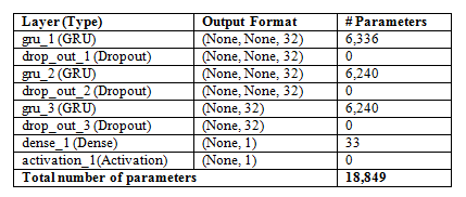
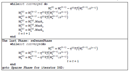
The model of 3 hidden layers with GRU using DSD training is shown in Figure 7. The recommended configuration of the DSD-3hGRU model is described in Table 3. The detailed training procedure is described in Algorithm 3.

Figure 7. Hybrid DSD-3hGRU model

Table 3. . Configuration of the proposed 3 hidden-layer DSD-3hGRU model

Algorithm 3.. DSD-GRU training procedure

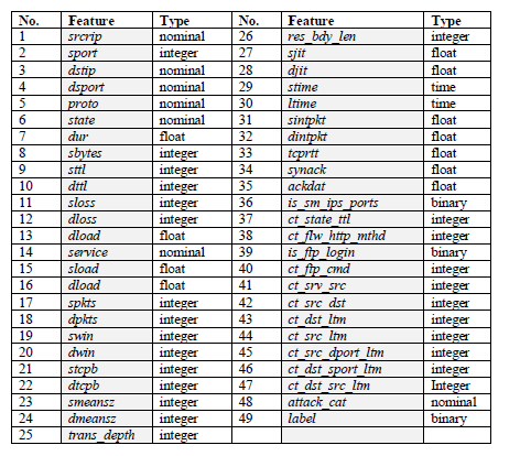
Table 4.. Features of the UNSWNB-15 dataset

4.2 Data Preprocessing

4.2.1 Convert nominal feature to numeric form

The process of converting nominal features into numeric form is called Numericalization. In the UNSW-NB15 dataset, there are 40 numeric features and 4 nominal features. Since the input value of RNN, LSTM, GRU must be a numeric matrix, we have to convert some nominal features, such as “proto”, “service” and “state” into numeric form. We convert these sets of numbers using the scikit-sklearn LabelEncoder library [12]. For example, the proto feature in the dataset with non-identical values including tcp, udp, and rdp will be encoded with the corresponding label to the numbers 1, 2, and 3.

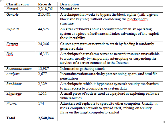
The dataset contains 10 types, one is normal and nine types of attacks (anomaly) including generics, exploits, fuzzers, DoS, reconnaissance, analysis, backdoor, shellcode, and worms. Table 5 shows the class classification details of the UNSW-NB15 dataset.

Table 5.Classification of attacks in the UNSW-NB15 dataset

4.2.2 Feature selection

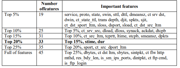
In [14], Malek Al-Zewairi and colleagues tested and found the most important features in the UNSW-NB15 dataset and showed the performance of the best model (i.e. the deep learning model using the top 20% set with a threshold of 0.4482) as shown in Table 6. Therefore, in this study, we reuse the Top 20% of the most important features for our experiments.

Table 6. Importance of features

4.2.3 Data Normalization Min-Max

Normalization is a scaling technique in which values are shifted and resized so that they end up between 0 and 1. Normalization requires that we know or be able to accurately estimate the minimum and maximum values that can be observed.

Because the scope of raw data is very wide and varied, in some machine learning algorithms, the objective function will not work properly if it is not normalized. Another reason for the feature normalization to be applied is that the prediction accuracy will increase compared to no normalization [15]. In this experiment, we use Min-Max normalization given by equation (13).

4.3. Experimental Environment

In this study, binary classification based on RNN, LSTM, GRU networks is selected. This model is trained on the comprehensive dataset UNSW-NB15. The algorithm is built on Python language and Keras library, Sklearn, runs on Tensorflow platform and Anaconda environment.

The experiment was performed on an Acer Nitro5 laptop, with a CPU configuration Intel Core i5-9300 2.4 GHz, 16 GB memory, and GPU 3 Gigabytes. Experiments have been designed to study the performance between 3 neural network models RNN, LSTM, and GRU in binary classification (normal, anomaly). The simple RNN, LSTM, and GRU models are the same, only differing in the core architecture of the neuron, specifically:

• The RNN/LSTM/GRU layers consist of 32 neuron units;
• Dropout layers has a dropout rate of 0.1;
• The Dense layer uses the sigmoid activation function.

In which, the Dropout layer helps to avoid overfitting, the last Dense layer is the output layer to evaluate the output as 1 or 0 (i.e. anomaly or normal). Each phase applies DSD to all 3 models DSD-3hRNN/DSD-3hLSTM/DSD-3hGRU. However, the final phase which is the re-dense phase restores the connections, the learning rate is reduced to 0.0001 in this phase.

5. RESULT EVALUATION

5.1. Evaluation Method

We use 5 common metrics to evaluate intrusion detection performance including Accuracy, Detection Rate, Precision, False Alarm Rate, and F1 score. Table 7 presents the confusion matrix including true positive (TP), true negative (TN), false positive (FP), and false negative (FN). TP and TN indicate that the attacked (anomaly) state and the normal state are classified correctly. FP indicates that a normal record is predicted incorrectly, i.e., the IDS warns of an unrealistic attack. The FN indicates that an attack record is incorrectly classified, i.e., the IDS does not warn and assume it as a normal record.

Table 7. Confusion Matrix

Accuracy –how close the measurements are to a particular value, representing the number of correctly classified instances of data over the total number of predictions. Accuracy may not be a good metric if the dataset is unbalanced (i.e. both negative and positive classes have different amounts of data). The formula calculating precision is defined in (14).

False Alarm Rate (FAR) – also known as False Positive Rate. This measure is calculated according to formula (15). The ideal ratio for this metric is as low as possible, i.e. the lower number of misclassifications is the better.

Precision –how close the measurements are. Precision is 1 only when numerator and denominator are equal (TP=TP+FP), this also means FP is 0. The formula calculating Precision is defined in (16).

Detection Rate (DR or Recall) –DR is 1 only if the numerator and denominator are equal (TP = TP + FN), this also means that the FN is 0. This criterion aims to evaluate the generalization of the found model and is determined by the formula (17).

We always expect both Precision and DR to be good, i.e. either the FP and FN values should be as close to zero as possible. Therefore, we need a measurement parameter that takes into account both Precision and DR, which is F1-score, determined by the formula (18).

F1-score is called a harmonic mean of the Precision and DR criteria. It tends to take the value closest to whichever is the smaller between the Precision and DR values. Therefore, the F1-score is a more objective representation of the performance of a machine learning model. Compared with the Accuracy, F1-score is more suitable to evaluate the instructive detection performance of unbalanced datasets.

5.2. Result and Evaluation

The training model is performed with the following cases:

• Case 1: RNN, LSTM, GRU model is trained on the UNSW-NB15 dataset.
• Case 2: RNN, LSTM, GRU model is trained on UNSW-NB15 dataset combined with DSD training scheme.

The above cases are all trained with Cross-validation [13], the sparsity parameter is 25, the epoch number is 10, and the batch_size is 32. The evaluation results are presented in Table 8 (case 1) and Table 9 (case 2). The evaluation criteria include Accuracy, FAR, Precision, Recall, and F1-score. Experimental results are listed in Table 8 and Table 9.

Table 8. Evaluation of RNN, LSTM, and GRU models on the UNSW-NB15

Table 9. Evaluation of DSD-3hRNN, DSD-3hLSTM, DSD-3hGRU on the UNSW-NB15

In Table 8, all three models have similar results in terms of accuracy. However, in terms of DR and F1-score, RNN gives the best results (91.0615% and 88.3684%). The FAR criterion shows that the multilayer neural network model GRU and LSTM give better results than the multilayer neural network model RNN (0.3711% and 0.3430% respectively, the smaller FAR, the better performance). Meanwhile, the GRU gives the best result in the Precision criterion with 92,4533%.

In Table 9, all three models have similar results in terms of accuracy. DSD-3hLSTM gives the best results in many criteria. Specifically, FAR is the lowest with 0.2619%, other criteria such as Precision, and F1-score are the highest at 94.1910%, and 88,5433%, respectively. For DR criteria, DSD-3hLSTM is equivalent to DSD-3hGRU.

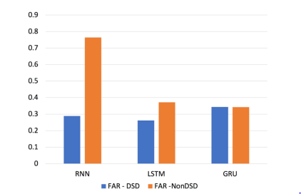
Figure 8. FAR comparison chart between RNN, LSTM, GRU with DSD and without DSD

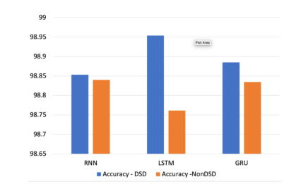
Figure 9. Accuracy comparison chart between RNN, LSTM, GRU with DSD and without DSD

With the results obtained in tables 10, 11, and 12, we see that combining the DSD training scheme with the hidden 3-layer neural network gives better results than the original models. Most of the criteria are improved as follows:

• The proposed model DSD-3hRNN: FAR (reduced by 0.4759%), Accuracy (increased by 0.0131%), Precision (increased by 7.6966%) compared with the original RNN neural network.
• The proposed model DSD-3hLSTM: FAR (reduced by 0.1092%), Accuracy (increased by 0.1927%), Precision (increased by 2.3928%), DR (increased by 1.8365%), F1-score (increased by 2.089%) compared with the original LSTM neural network.
• The proposed model DSD-3hGRU: Accuracy (increased 0.0503%), Precision (increased of 0.0773%), DR (increased of 1,0504%), F1-score (increased of 0.617 %) compared with the original GRU neural network model.

Table 10. Evaluation of the DSD-3hRNN and RNN on the UNSW-NB15 dataset

Table 11. Evaluation of the DSD-3hLSTM and LSTM on the UNSW-NB15 dataset

Table 12. Evaluation of DSD-3hGRU and GRU on the UNSW-NB15 dataset

For a simpler look, we extract results based on two key criteria (FAR and Accuracy) to show in Figures 8 and 9. With the FAR criterion, we found that DSD-3hRNN gives a significant improvement compared with the original model (reduced by 0.4759%). With Accuracy criterion, all 3 models are improved, but DSD-3hLSTM is improved the most (increased 0.1927%).

RNN has a problem with “vanishing gradient” (gradient is used to update the value of the weight matrix in RNN and it gets smaller layer by layer when done show back propagation). When the gradient becomes very small (value is close to 0) then the value of the weight matrix will not be updated further and hence the neural network will stop learning at this layer. However, when using DSD, the RNN will be weighted and retrained again. This helps to restore the weights, overcomes the “vanishing gradient” problem, and increases the training efficiency in the final Dense phase. Meanwhile, LSTM has added ports (forget port, update gate and tanh function) to overcome the problem of “vanishing gradient”, so the intrusion detection efficiency of LSTM by DSD training is better improved when DSD is applied to the RNN. However, because GRU is the proposed model to simplify the architecture of the LSTM model. It uses the update port to replace the input and forget ports. This simplification of the architecture helps GRU improve the learning time, but the efficiency level is not equal to the LSTM.

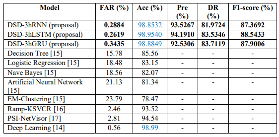
Besides, we also collect results from other studies [16], [17], [18], and [19] to compare with our results. The results in Table 13 show that our proposed solution has better performance in many criteria in detecting network intrusion than previous studies as follows:

• The accuracy of the proposed model DSD-3hRNN is 98,8532%, DSD-3hLSTM is 98,9541%, and DSD-3hGRU is 98,8849%.
• The false alarm rate of the proposed model DSD-3hRNN is 0.2884%, DSD-3hLSTM is 0.2619%, DSD-3hGRU is 0.3435%.
• For the remaining criteria (Precision, DR, F1-score), we did not collect corresponding data for comparison.

Table 13. Performance comparison of the proposed training model with other studies

Thus, the false alarm rates of the 3 proposed models are quite good, much lower than that of other proposed models. The accuracy of the proposed model is equivalent to Deep Learning [14] and higher than the remains [15, 16, 17]. In general, harmonizing the criteria, the DSD-3hLSTM training scheme gives the best result in the 3 proposed models with False Alarm Rate of 0.2619%, Accuracy of 98.954%, Precision of 94.1910%, F1-score of 88.5433%.

6. Conclusions

This paper presented a method to improve the performance of intrusion detection systems by integrating big data technologies and deep learning techniques. UNSW-NB15 dataset is used to evaluate the proposed approach. We proposed the hybrid model of a hidden 3-layer neural network with the DSD training scheme: Hybrid DSD-3hRNN model, Hybrid DSD-3hLSTM model, Hybrid DSD-3hGRU model. In the experiment, three proposed models are trained with sparsity parameters of 25, batch_size of 32. The evaluation criteria are: Accuracy, FAR, Precision, Recall and F1 Score. All experiments are conducted on Anaconda environment with the Keras & TensorFlow 2.The results obtained in tables 10, 11, and 12, we see that combining the DSD training scheme with the hidden 3-layer neural network gives better results than the original models.

The novelty in our proposed model is there as on able number of hidden layers chosen to solve both under-fitting and over-fitting problems that most deep learning models have to face. However, there are still some limitations in experimenting and evaluating the proposed model. We have to check many times to find the appropriate parameter, such as the value of the sparsity parameter, the number of hidden layers, the number of neurons per layer. In addition, we do not have a complete assessment of the experimental time.

The next research will be studying the DSD scheme to find the appropriate set of parameters (epochs, learning rate, sparsity) and activation functions (reLU, Leaky ReLU, Swish, etc.) to improve the instructive detection efficiency. Besides, to index the specific type of attack, we also intend to study the DSD training scheme merged with deep neural networks such as CNN, DNN using other attack datasets including labeled and unlabeled records.

Conflicts of Interest 

The authors declare no conflict of interest.

References 

[1]     Hettich, S. and Bay, S. D., “KDD Cup 1999 Data” 28 October 1999. [Online]. Available: http://kdd.ics.uci.edu. [Accessed 02 Feb 2020].

[2]     M. Tavallaee, E. Bagheri, W. Lu, and A. Ghorbani, “A Detailed Analysis of the KDD CUP 99 Dataset”, 2009. [Online]. Available: https://www.unb.ca/cic/datasets/.

[3]     Nour Moustafa, Jill Slay, “UNSW-NB15: A Comprehensive Dataset for Network” in Military Communications and Information Systems Conference (MilCIS), Canberra, Australia, 2015.

[4]     Moustafa, Nour Moustafa Abdelhameed, “The UNSW-NB15 Dataset Description” 14 November 2018. [Online]. Available: https://www.unsw.adfa.edu.au/unsw-canberra-cyber/cybersecurity/ADFA-NB15-Datasets/. [Accessed 02 August 2020].

[5]     Vinayakumar R et al., “A Comparative Analysis of Deep learning Approaches for Network Intrusion Detection Systems (N-IDSs)” International Journal of Digital Crime and Forensics, vol. 11, no. 3, p. 25, July 2019.

[6]     Song Han∗, Huizi Mao, Enhao Gong, Shijian Tang, William J. Dally, “DSD: Dense-Sparse-Dense Training For Deep Neural Networks” in ICLR 2017, 2017.

[7]     Mohammed Awad1 and Alaeddin Alabdallah, “Addressing Imbalanced Classes Problem Of Intrusion Detection System Using Weighted Extreme Learning Machine”, International Journal of Computer Networks & Communications (IJCNC), Vol.11, No.5, 2019

[8]     Saad Al-Ahmadi1 and Yasser Alharbi A deep learning technique for web phishing detection combined url features and visual similarity, Journal of Computer Networks & Communications (IJCNC), Vol.12, No.5, September 2020

[9]     Anani, Wafaa, “Recurrent Neural Network Architectures Toward Intrusion Detection” in Recurrent Neural Network Architectures Toward Intrusion Detection, Electronic Thesis and Dissertation Repository. 5625, 2018.

[10]   K. Cho, J. Chung, C .Gulcehre, and Y. Bengio, “Empirical evaluation of gated recurrent neural networks on sequence modeling” Computing Research Repository (CoRR), 2014.

[11]   Brownlee, Jason, “Overfitting and Underfitting With Machine Learning Algorithms” 12 August 2019. [Online]. Available: https://machinelearningmastery.com/overfitting-and-underfitting-with-machine-learning-algorithms/. [Accessed 03 August 2020].

[12]   Gupta, Prashant, “Cross-Validation in Machine Learning” Towards Data Science, 05 June 2017. [Online]. Available: https://towardsdatascience.com/cross-validation-in-machine-learning-72924a69872f. [Accessed 02 August 2020].

[13]   Brownlee, Jason, “Gentle Introduction to the Bias-Variance Trade-Off in Machine Learning” 25 October 2019. [Online]. Available: https://machinelearningmastery.com/gentle-introduction-to-the-bias-variance-trade-off-in-machine-learning/. [Accessed 03 August 2020].

[14]   Pedregosa et al., “Scikit-learn: Machine Learning in Python” 2011. [Online]. Available: https://scikit-learn.org/stable/modules/.

[15]   Sergey Ioffe, Christian Szegedy, “Batch Normalization: Accelerating Deep Network Training by Reducing Internal Covariate Shift”, Computer Science – Machine Learning, 2015.

[16]   Malek Al-Zewairi, Sufyan Almajali, Arafat Awajan, “Experimental Evaluation of a Multi-Layer Feed-Forward Artificial Neural Network Classifier for Network Intrusion Detection System”,The 2017 International Conference on New Trends in Computing Sciences, At Amman, Jordan, 2017.

[17]   N. Moustafa and J. Slay, “The evaluation of network anomaly detection systems: Statistical analysis of the UNSW-NB15 dataset and the comparison with the KDD99 dataset”, Information Security Journal: A Global Perspective, Jan 2016.

[18]   Seyed Mojtaba Hosseini Bamakan, H. Wang, and Y. Shi, “Ramp loss k-support vector classification-regression; a robust and sparse multi-class approach to the intrusion detection problem”,Knowledge-Based Systems, vol. 126, pp. 113-126, 2017.

[19]   P. Mishra, E. S. Pilli, V. Varadharajan, and U. Tupakula, “PSI-NetVisor: Program semantic aware intrusion detection at network and hypervisor layer in cloud”, Journal of Intelligent &Fuzzy Systems, vol. 32, p. 2909–2921, 2017.

Authors

Trong Thua Huynh is currently the Head of Information Security Department, Faculty of Information Technology, Posts and Telecommunications Institute of Technology in Ho Chi Minh City, Vietnam. He received a Bachelor’s degree in Information Technology from Ho Chi Minh City University of Natural Sciences, a Master degree in Computer Engineering at Kyung Hee University, Korea, and a Ph.D. degree in Computer Science at the Ho Chi Minh City University of Technology, Vietnam National University at Ho Chi Minh City. His key areas of research include Information Security in IoT, Blockchain, Cryptography, and Digital Forensics.

Hoang Thanh Nguyen is currently the Lecturer in Ho Chi Minh City, Vietnam. He received a Master’s Degree in Information Systems from the Institute of Post and Telecommunications Technology. His research areas are Information Security, Machine Learning.