IJCNC 02

MULTIMODALQOS AWARE LOAD BALANCED CLUSTERING IN 5G-ENABLED IOT SENSOR NETWORK

Biswanath Dey 1 , Sukumar Nandi 2 , Sivaji Bandyopadhyay 3 and Samir Borgohain 1

1 Department of CSE, National Institute of Technology, Silchar, India

2 Department of CSE, Indian Institute of Technology, Guwahati, India

3 Department of CSE, Jadavpur University, Jadavpur, India

ABSTRACT

Formation of balanced clusters in IoT-based wireless sensor networks constitutes an NP-hard problem for which no straightforward solution exists. Existing approaches often employ centralized schemes with significant communication overhead or rely on computationally intensive evolutionary algorithms, which limit their practical applicability. To address this challenge, we introduce two simple yet efficient distributed methods: the Load Balanced Greedy Cluster Assignment (LBGCA) for large-scale IoT networks, and its extension, the Multi-modal Load Balanced Greedy Cluster Assignment (MLBGCA) for QoS–aware applications. Both algorithms adopt a localized greedy strategy that minimizes communication overhead by requiring only neighbourhood-level information. LBGCA enables nodes to self-organize into balanced clusters, whereas MLBGCA integrates application-specific QoS constraints by dynamically adjusting cluster head load profiles. Simulation results across grid, Gaussian, and random deployments demonstrate that LBGCA reduces load imbalance by 20–40% and energy consumption by 70–90%, while MLBGCA further improves load imbalance by 30–50% and decreases energy use by 60–90% relative to existing algorithms.

KEYWORDS

IoT sensor network, 5G, Energy efficiency, Distributed algorithm, Localized greedy load balancing, QoS
aware load balancing, Multi modal load balancing.

1. INTRODUCTION

The evolution of 5G networks is transforming communication technologies by enabling faster data transfer and supporting large-scale applications such as the Internet of Things (IoT) [1]. One of the most promising applications of 5G’s massive machine-type communications (mMTC) is the deployment of distributed wireless sensor networks (DWSNs), widely used for monitoring and detection tasks. In such networks, each sensor node operates with limited processing power, transmission range, and battery capacity. These restrictions make energy efficiency and scalability critical issues for extending the lifespan of wireless sensor networks (WSNs), which serve as the perceptual layer of large-scale IoT infrastructures [2].

Clustering has emerged as a key strategy to mitigate these constraints [3,26,27]. By organizing nodes into clusters with designated heads (CHs) for data aggregation, this approach reduces redundant transmissions and improves energy efficiency. A typical hierarchical communication framework is illustrated in Fig 1. Despite its benefits, the CH role consumes significantly more energy [11]. While CH rotation helps distribute this load, it often fails to achieve true balance, leading to network instability, coverage gaps, and premature partition [24,30]. The problem is further complicated by the NP-hard nature of forming optimally balanced clusters [5,33].

Existing solutions often struggle with this complexity. Centralized schemes [35] and heuristic or evolutionary algorithms —including nature-inspired methods like Grey Wolf Optimizer—can improve energy distribution but introduce substantial computational and communication overhead, making them unsuitable for resource-constrained nodes [4,5,8,22]. Similarly, techniques like compressive sensing and soft-k-means clustering show promise but are limited by their complexity and reliance on global information [9,16]. Furthermore, the diverse QoS requirements of different IoT applications (e.g., latency for surveillance, reliability for habitat monitoring) mean no single strategy is universally optimal [10,12,28]. This creates a clear need for lightweight, adaptive, and distributed clustering methods that can balance energy load without significant overhead while meeting application-specific QoS demands [14,15,29].

To address this gap, we propose two lightweight, distributed algorithms for load-balanced clustering. The first, Load Balanced Greedy Cluster Assignment (LBGCA), uses localized neighbourhood information and minimal messaging to form balanced clusters via a greedy method. The second, Multi-modal Load Balanced Greedy Cluster Assignment (MLBGCA), extends LBGCA by integrating application-specific QoS constraints through multimodal load profiling of CHs. Together, these algorithms provide energy-efficient, scalable, and QoS-aware clustering for diverse IoT deployments.

The remainder of this paper is structured as follows: Section 2 defines the problem and reviews related work. Section 3 details proposed LBGCA algorithms, and section 4 analyzed its performance. Section 5 describes multi modal load balancing scheme and MLBGCA algorithm. In section 6 performance of our proposed algorithms are detailed. Finally, section 7 concludes the paper.

2. RELATED WORKS

Forming load-balanced clusters in WSNs and IoT is an NP-hard problem, necessitating heuristic and meta-heuristic solutions aimed at maximizing network longevity by evenly distributing the energy burden of Cluster Heads (CHs) [18, 20, 25, 31, 41]. Research has evolved from simple probabilistic methods to more sophisticated algorithms [45].

Early protocols, such as the seminal LEACH [3], established CH rotation to prevent node burnout. While innovative, its stochastic nature led to suboptimal clusters. Enhancements like ILEACH [6] incorporated residual energy and distance, but the core probabilistic approach still lacked a guarantee for balanced cluster sizes [6].

Subsequent metric-based algorithms sought more deterministic control. Protocols like LBC [4] used geographical positioning to minimize cluster size disparities, while NLDLB [9] assigned nodes based on local density rules. These methods improved balance but introduced overheads like localization costs and lacked adaptability [4, 9]. 

The pursuit of near-optimal solutions led to bio-inspired and centralized optimization techniques, such as Genetic Algorithms (GAs) [7,8,40]. While capable of high-performance clustering, their non-deterministic nature and high computational complexity relegate them to a centralized base station, creating a single point of failure and significant communication overhead [7, 8, 19]. 

In parallel, distributed protocols [17,21] emerged to minimize overhead and enhance scalability[37]. Algorithms like DLBCA [12] and CALB [49] use local information (e.g., residual energy, neighbour proximity) for independent CH election, achieving low overhead [12, 13, 49]. However, a critical limitation of these approaches is their narrow definition of “load,” which is predominantly based on cluster size and residual energy, overlooking the quality of the onward multi-hop path to the base station.

Recognizing that cluster size is an insufficient metric, later work incorporated more nuanced strategies. DEACP [47] managed intra-cluster traffic with sleep scheduling, HRLBP [50] used mobile data collectors, and other methods employed Vice-Cluster Heads [51] or multi-level heterogeneity [42]. While these advanced load management, they largely side stepped the integration of application-specific Quality of Service (QoS) parameters like latency and reliability into the core load-balancing decision [47, 50]. Non-clustered approaches like ORR [32] also face significant overhead from centralized control. 

A comparative analysis of these protocols (summarized in Table 1) reveals a clear taxonomy of trade-offs. Centralized and bio-inspired algorithms achieve high performance at the cost of impractical overhead, while distributed algorithms offer scalability but use an oversimplified load model that ignores both the onward path to the sink and application-level QoS. 

This leaves a pronounced gap for a practical, distributed solution that employs a low-complexity strategy to achieve load balancing based on a multi-modal assessment of load, incorporating not just energy and cluster size, but also the critical QoS parameters demanded by modern IoT applications. Our proposed LBGCA and MLBGCA algorithms are designed to fill this gap.

3. LOAD BALANCED GREEDY CLUSTER ASSIGNMENT (LBGCA)

We first propose a lightweight and distributed strategy for cluster formation we call Load Balanced Greedy Cluster Assignment (LBGCA) algorithm. LBGCA prioritizes load balancing with minimal complexity. 

3.1. System Assumptions  

The network comprises several sensor nodes and a few coordinator nodes (Cluster Heads, CHs). Communication occurs over wireless links within a fixed range. We assume node positions are known, typically via GPS. Each sensor node greedily selects the CH with the fewest existing members, thereby promoting balanced cluster sizes.

3.2.The LBGCA Algorithm 

The detailed pseudo code for LBGCA is decribed in Algorithm 1. For every sensor node, the algorithm initializes two key variables namely, ‘points_con’ (the minimum number of members a candidate CH has) and ‘dist’ (the Euclidean distance to the nearest candidate CH). At start both ‘points_con’ and ‘dist’ are set to a high initial value. The node then identifies all CHs within its communication range. The assignment follows a two-tiered rule set. Primary Rule (Load): The sensor node is assigned to the CH with the fewest current members. Tie-Breaker Rule (Proximity): If multiple CHs have the same smallest number of members, the node selects the closest one (i.e., the CH with the minimum Euclidean distance, path_dist). Once a member joins a CH, the assigned counter for the selected CH is incremented.

Table 1. Comparative analysis of load balancing algorithms

4. PERFORMANCE EVALUATION OF LBGCA

To evaluate the efficacy of LBGCA algorithm, we compared it against classic load balancing protocols (LBC [4], EELBCA [20]) and some more recent approaches like (LLALBC [13], DEACP [47]) using MATLAB Simulink [54]. Simulations were conducted under varied network conditions to assess performance in terms of load balance and energy efficiency.

4.1.Simulation Setup

We modelled multiple network scenarios with 50, 100, and 150 sensor nodes distributed across areas of 50×50, 100×100, and 150×150 units, respectively. Two primary node distribution models were employed: uniform normal distribution, and Gaussian grid-based distribution. Normal distribution is applicable typically for broad-area monitoring. Gaussian grid-based distribution is more suitable for applications that require focused coverage on specific points of interest [34, 36]. Performance metrics compared are, standard deviation of cluster sizes (indicating load balance), average energy consumption across all nodes, and network lifetime until the First Node Death (FND) and Last Node Death (LND) [23, 43].

4.2.Performance of LBGCA and Analysis

Fig. 2 and Fig.3 shows the load balancing performance of LBGCA for normal node distribution and grid-based node distribution, respectively. LBGCA consistently achieves a lower standard deviation in CH load compared to all benchmarks across various network scales and topologies. This improvement is a direct result of LBGCA’s core mechanism, which explicitly monitors and minimizes the number of members per CH during cluster formation. Furthermore, LBGCA demonstrates better energy efficiency, as depicted in Fig. 4 and Fig. 5. In all tested scenarios, LBGCA maintained lower average energy consumption over multiple operational rounds. This advantage stems from the algorithm’s simplicity, which relies on minimal localized message passing and avoids the computational overhead of more complex methods.

Figure 2. Standard deviation in CH load (Normal random distribution of node

Figure 3. Standard deviation in CH load (Grid based distribution of nodes)

4.3.Limitations and Motivation for Multi-Modal Profiling

Despite its strengths, LBGCA, defines cluster head “load” solely by the count of member nodes, as like the benchmarks it outperforms. This simplistic metric ignores critical application- specific Quality of Service (QoS) factors[38,53]. For instance: A CH with few members may lack sufficient energy for the onward multi-hop transmission to the base station. Again, a CH may be unable to relay data within a required latency bound due to congestion on its path. Therefore, a more comprehensive load model is necessary. This motivates our next enhanced algorithm, which incorporates a composite multi-modal load profile for each CH, considering key factors like residual energy, path viability, and service parameters, while retaining a low-complexity greedy assignment methodology. We detail this modified algorithm in the following section.

Figure 4. Mean(Avg.) energy consumption (100*100 network, 50 nodes)

Figure 5. Mean(Avg.) energy consumption (200*200 network, 100 nodes)

5. MULTI MODAL LOAD BALANCED GREEDY CLUSTER ASSIGNMENT (MLBGCA)

MLBGCA algorithm meticulously performs the QoS aware cluster formation based on the prospective cluster head’s Composite Multi-modal Load characteristics Profile (CMLP).

5.1. Components of Composite Multi Modal Load Characteristic Profile of Prospective CHs (CMLP)

To compute the prospective cluster head’s Composite Multi-modal Load characteristics Profile (CMLP) the following key parameters taken in to consideration.

5.1.1. Number of Neighbors (NN)

NN is defined as the total number of neighboring nodes of prospective CH, that is, the quantity of sensor nodes that the current cluster head will service in the subsequent rounds of network operation. NN is calculated as follows Each prospective CHs maintains a counter NN initialized to zero. During the cluster setup phase, each CH broadcasts an ADVertisement packet with a preset power level. The non cluster nodes who are within the communication range of multiple CHs may receive multiple ADV packets from different CH nodes. Each non cluster head node sends their JOIN request to all CH nodes that are within the feasible radio range of the non CH node. Note that a non CH node may have received m number of advertisement messages, but it may not have sufficient energy to sends its data packets to feasibly to reach all m such CHs. So the non CH nodes on receiving the ADV packets, sends their JOIN request to a subset of CH nodes in its proximity from which it received the ADV packets, ordered by the distance of the CH node from itself calculated based on the RSSI (the received signal strength indicator) of the ADV packets. On receiving JOIN request from each non CH nodes, the cluster head node (CH) increments its NN count by 1. NN oriented load profile (LP1) escalates by an application-specific characteristic load factor viz. α with the augmentation of nodes inside the current cluster.

5.1.2. Residual energy profile (REP) of Prospective CH

Considering as the energy required by the transceiver circuitry to process 1 bit of information, the amount of energy expended by CH node to receive k bit data packets n number of cluster member nodes can be computed as:

Each CH needs to collect the data packets from the potential members within the cluster, thereafter aggregate the n data packets if the application demands and then send the aggregated packet towards next hop on the path to the base station. Depending on the number of neighbors or number of cluster member nodes to be serviced the CH can estimate the amount of energy to be expended for receiving m number of packets from m member nodes. If the current application requires in network data aggregation, the CH can estimate the amount of energy required for data aggregation.

Combining the above energy consumption estimates the CH compares its current remaining energy and computes its REP as follows:

REP = Current Remaining energy – (Sum of energy required for reception of packets from m member nodes, energy required for data aggregation)

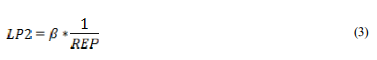
The REP-oriented component of the load profile, referred to as LP2, increases proportionally with an application-specific parameter β as the remaining energy of a potential cluster head decreases. The parameter β is influenced by factors such as the nature of the application, transceiver hardware characteristics, and the region of interest (ROI).

5.1.3. Base Station (BS) Distance or Next Hop Node Distance Towards BS from Prospective CH (DIST)

The component load profile LP3 increases by an application specific factor when the distance of the potential Cluster Head from BS increases or the distance of next of node down line to the Base Station increases. The parameter γ is determined by factors such as distance dispersion, channel variability, and shadowing effects associated with wireless communication within the region of interest (ROI).

Upon reception of data packets from different cluster member(s) and aggregating if application demands, the CH needs to transmit the aggregated packets to the next hop CH towards BS. The CH can estimate the amount of energy required for successful transmission of the aggregated data packet from its distance from the next hop node on the different paths towards the base station. On receiving data packets from the cluster member nodes, each cluster head node must have sufficient energy to process and transmit the packet to next hop nodes towards the sink for the path to be feasible.

The amount of energy expended to transmit k-bit data packet over a distance d can be calculated as follows:-

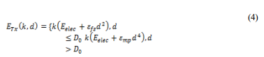
Where Eelec is the ambient energy dissipation in relaying node E_fs  and  E_mp circuitry, and are the path loss coefficients for line of sight propagation and multi path propagation respectively.

While the energy required collecting a k-bit packet is:

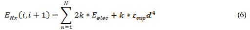
Thus the total energy needed to forward a k-bit packet in from ith hop to (i+1)th on a multi hop path towards destination can be computed as:

If DIST is the distance from CH to its next hop relay node in the path towards the sink node, amount of load component is estimated as:-

Here, γ is an application-specific parameter influenced by factors such as deployment distance spread, channel interference, and potential wireless shadowing effects within the deployment region

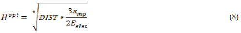
For a given DIST the optimal number of hops can be computed using the following equation:

5.1.4. Prospective Path Delay (PD)

Component load profile LP4 with respect to path delay (PD) increased by an application specific factor δ as the prospective path to the base station via the CH increases. Some specific application like video surveillance often requires the sensed information packet to be transmitted to the base station within the bounded delay. Path delay in itself may comprises of packet propagation delay, packet processing time required at the CH and delay involved in the Queuing of the packets at the CH.

While wireless channel propagation delay, packet processing time required by the electronics circuitry at the CH can be estimated beforehand and almost remain constant, the queuing delay remain dynamic and temporally depends on the number of neighbours being served by the CH as well as packets generation rate at the member nodes. This can be estimated dynamically by the number of packets still waiting to be processed at a particular time. Combining the above CH calculates its LP component as follows,

PD = Packet size * (Wireless propagation delay/bit + Processing time required/bit) + Estimate of
queuing delay,

Thus, we calculate corresponding LP component as,

5.1.5. Forward link & path reliability (FLR & FPR)

Reliability of next hop communication link in the path towards the Sink [46] is one of the most important factors for successful transmissions for achieving high throughput and avoiding retransmission of packets due to packet loss. Thus, forward link reliability or FLR can be formulated as the joint probability of successful packet transmission by the CH and subsequently reception of the acknowledgement packet by the CH corresponding to the transmitted packet.

Thus, FLR can be measured as follows:-

FLR = probability of successful transmission of packet by the CH to its next hop neighbour towards the path to base station * probability of successful reception of the acknowledged packet If there are m number of relay nodes from the CH to sink or base station on the path towards the base station, then forward path reliability (FPR) can be calculated as,

FPR = sum of all FLR

Based on the above observation, Load profile (LP) of a node in decreased by a factor for the higher value of FPR that is if a particular path from this CH to the Sink is more reliable. The load component for forward link/path reliability is calculated as:

5.1.6. Computation of Composite Multi modal Load Profile (CMLP)

Based on the above load factors calculation for the prospective cluster head we can formulate the composite multi modal load profile (CMLP) as follows:-

C₁ through C₅are the coefficients to be used to enumerate the weightage to particular load profile factor depending upon the application demand.

5.2. CMLP based Greedy Load balanced Clustering algorithm

For the purpose of assigning Cluster Heads to individual nodes who are not members of the CH, we present a straightforward and greedy strategic approach based on the Composite Multi modal Load characteristic Profile (CMLP) of each potential cluster head candidates. A ‘Feasible CMLP’ is determined by dividing the network’s total current capacity by the number of cluster heads. We iteratively identify the potential cluster heads within the range of transmission of every node in the network and assign each node to a CH with minimum CMLP dynamically based on the current network state

Algorithm 2 outlines the complete procedure for MLBGCA. The variable NearestCH represents the shortest distance between a given sensor node and its selected cluster head, whereas Neighbors refers to the highest number of sensor nodes connected to cluster heads that fall within the communication range of the current sensor.

The MLBGCA algorithm starts by initializing the variables ‘NearestCH’ and ‘Neighbors’ with large placeholder values. When a cluster head (CH) is found within the transmission range of a sensor node and has fewer connected sensors than the current Neighbours threshold, the sensor is assigned to that CH—provided the CH’s feasible CMLP (Composite Multimodal Load Profile) remains within permissible bounds, and the CMLP is updated accordingly. If the CH’s CMLP exceeds the threshold, the sensor connects to that CH only if no other CH exists within its transmission range. In cases where multiple CHs are within range, the one with the lowest current CMLP is selected for assignment. After each successful node assignment, the CH checks whether its CMLP still falls within acceptable limits. If the updated CMLP surpasses the permissible value, the CH broadcasts this change to its neighbouring nodes.

6. RESULTS &DISCUSSION

To study the effectiveness and efficacy of our algorithm, MLBGCA we compared it with similar widely quoted classic hybrid load balancing algorithms viz. HRLBP[50] and two recently published & widely quoted algorithms, viz. LLALBC [13], and CALB[49] for similar network conditions in Matlab [54]. Simulations were carried out across multiple network scenarios using different node deployment distribution functions, namely Uniform, Gaussian, and grid-based layouts. For each scenario, separate deployments of 50, 100, and 150 sensor nodes were tested within network areas of 100×100, 200×200, and 250×250 units, respectively, in accordance with the chosen distribution models.

For calculating CMLP we have taken simple values for equals to 0.50 though they can be best measured from different application experience[38,39,52], and for load coefficients C1 through C5 for generalization we have taken value as equals to 0.20 giving equal weightage to all load factors. We use the following metrics [43,44,48] as defined for performance evaluation of our algorithm, (i) Variation in load distribution across various cluster heads, (ii) Average Energy expenditure at different stages of operational network, (iii) Average throughput, (iv) Packet delivery ratio (PDR) that is average number of packets delivered with respect to average number of packets generated in different algorithms, (v) End to end packet transmission delay, that is time required for delivering data packets to base station with respect to total number of packets delivered to base station by different protocols, and (vi) Network stability period that is rounds of network operation achieved by different protocols until the first node dies

 Fig. 6 and Fig. 7 illustrate the standard deviation across CH load distributions for different node deployment distributions viz. Uniform distribution, and Gaussian distribution. Our algorithm demonstrates a significant reduction in the standard deviation of cluster head load across various network types. Because our technique explicitly monitors and restricts the total members entering into the cluster during cluster formation, the variance in cluster load is also far lower than with existing algorithms.

Figure 6. Standard deviation of CH load with normal distribution of deployment

Figure 7. Standard deviation of CH load with Gaussian distribution of nodes

Fig. 8 and Fig. 9 show the average energy consumption of sensor nodes over multiple rounds of operation for two distinct setups: a 200×200 grid network with 100 nodes and a 250×250 grid network with 150 nodes, respectively. Across all scenarios, our approach consistently outperforms existing algorithms in terms of energy efficiency. This improvement stems from our protocol’s use of accurately computed load profiles for cluster head selection, rather than relying solely on the number of connected members. Additionally, the algorithm maintains minimal localized message overhead, ensuring effective load-balanced cluster assignments.

Average Throughput in different protocols for different communication range of the nodes different distributions for 200×200 network with 100 nodes, is analysed and reported in Fig. 10 and Fig. 11. Throughput increases with all protocols with increasing communication range. However due to efficient and reliable weighted load profile based cluster assignment in our CMLP algorithm average throughput is substantially higher in all cases than the other protocols for both normal and Gaussian distribution of node deployment.

Fig. 12 and Fig.13 shows the average end-to-end delay in different protocols, for both normal and Gaussian distribution of node deployment. There is a general trend seen that average delay minimizes with increasing number of nodes in the network if with keep the communication range constant. This is possibly because number of next hops for any CH to send a packet to base station minimizes, as the probability of finding a node for next hop at an optimum position increases with increasing number of nodes in the network. Also as MLBGCA takes into account the congestion and queuing delay for all the prospective paths towards the base station from each CH to calculate load profile for each CH to find always the best path from multiple available path, delay in case of MLBGCA is always found to be lower than the other classical protocols.

Figure 8. Mean (Avg.) energy consumption [network size 200*200, 100 nodes]

Figure 9. Mean (Avg.) energy consumption [network size 250*250, 150 nodes]

Fig 14 illustrates packet delivery ratio for different protocols at different stages of network operation when all, three forth, half, and one fourth of the nodes alive in the network. Although PDR decreases with decreasing number of alive nodes, in MLBGCA we get higher PDR in all cases with respect to other protocols. This is because MLBGCA also takes into account the both forward and reverse link vis-à-vis path reliability to compute the load profile of the CHs and the best path is always selected as the nodes selects the CHs with lowest load following the simple but effective greedy algorithm.

Figure 10. Avg. throughput for different protocols, normal distribution, network size 200*200

Figure 11. Avg. throughput in different protocols, Gaussian distribution, network size 200*200</p>

Figure 12. Avg. end-to-end delay in different protocols, normal distribution of nodes in network of size 250*250

Figure 14. Packet Delivery Ratio (PDR) at varying percentages of alive nodes in a 250 × 250 network area with 150 deployed sensor nodes.

Fig. 15 reveals the network stability period in different protocols for normal distribution of nodes in network of size 250*250. Similar results obtained in Gaussian distribution of nodes also. It is observed that as MLBGCA takes into account various factors meticulously like number of neighbors, remaining energy, distance, path delay and link reliability to form a composite load profile for the Cluster heads and as the normal member nodes always choose the best CH from within their range to forwards their data packets following a simple greedy assignment the average energy consumption of the network nodes always lower in case of MLBGCA. This has a direct impact on the network stability period as it is seen that maximum number of nodes remained alive in case of MLBGCA for almost 80% of the entire effective network lifetime until the network got disconnected. Also the total number of nodes died always remained lower in case of MLBGCA with respect to other classic load balancing protocols.

7. CONCLUSION &FUTURE WORK

This paper introduces a straightforward yet effective greedy algorithm designed for multimodal load balancing in a cluster-based 5G IoT sensor network, aiming to enhance energy efficiency and ensure balanced workload distribution among cluster heads. In our first algorithm we use the one hop neighbourhood information to perform well balanced cluster formation using solely localized information without any global knowledge of the network. Subsequently in our modified algorithm we proposed a framework to compute efficient composite multi modal load profile of CH node and use simple and localized greedy approach not only to achieve well balanced cluster but also to support application specific QoS demand for advanced applications like multimedia traffic and video surveillance applications for 5G IoT based clustered sensor network.

Figure 15. Network stability period in different protocols, Normal distribution of nodes in network of size 250*250

We have tested our algorithm on various node distributions and different network scenario to evaluate its efficacy. While the cluster is being formed, our algorithm significantly reduces the variance of load among the CHs by assigning members to cluster head nodes in a simple yet efficient manner.

Additionally, our algorithm does not employ centralized or global network information; rather, it establishes a load-balanced cluster based on minimal local information. Experimental results on different network setup show that our algorithms significantly out perform the existing algorithms in terms of energy usage, delay, PDR and throughput. The fact that our technique doesn’t rely on computationally intensive algorithms makes it suitable for usage with both homogeneous and heterogeneous sensor networks. Further investigation into other application domains and networks with distinct deployment patterns, such as linear, c-shaped, and y-shaped networks, will allow us to optimize application-specific composite load parameters estimation in our future work.

CONFLICT OF INTEREST

The authors declare no conflict of interest.

ACKNOWLEDGEMENTS

The authors would like to thank everyone, just everyone!

REFERENCES

[1] L. Atzori, A. Iera, and G. Morabito, “The Internet of Things: A survey,” Comput. Netw., vol. 54, no. 15, pp. 2787–2805, Oct. 2010

[2] I. F. Akyildiz, W. Su, Y. Sankarasubramaniam, and E. Cayirci, “A survey on sensor networks,” IEEE Commun. Mag., vol. 40, no. 8, pp. 102–114, Aug. 2002

[3] W. B. Heinzelman, A. P. Chandrakasan, and H. Balakrishnan, “An application-specific protocol architecture for wireless microsensor networks,” IEEE Trans. Wireless Commun., vol. 1, no. 4, pp. 660–670, Oct. 2002

[4] G. Gupta and M. Younis, “Load-balanced clustering of wireless sensor networks,” in Proc. IEEE Int. Conf. Commun. (ICC), Anchorage, AK, USA, May 2003, vol. 3, pp. 1848–1852

[5] Biswanath Dey, Sivaji Bandyopadhyay, and Sukumar Nandi, Mobility Assisted Adaptive Clustering Hierarchy for IoT Based Sensor Networks in 5G and Beyond, Journal of Communications, vol. 18, no. 6, pp. 346-356, June 2023

[6] N. Kumar and J. Kaur, “Improved LEACH protocol for wireless sensor networks,” in Proc. 7th Int. Conf. Wireless Commun., Netw. Mobile Comput. (WiCOM), Wuhan, China, Sept. 2011, pp. 1–5

[7] P. Kuila, S. K. Gupta, and P. K. Jana, “A novel evolutionary approach for load balanced clustering problem for wireless sensor networks,” Swarm Evol. Comput., vol. 12, pp. 48–56, Apr. 2013

[8] P. Kuila and P. K. Jana, “A novel differential evolution based clustering algorithm for wireless sensor networks,” Appl. Soft Comput., vol. 25, pp. 414–425, Dec. 2014.

[9] J. Zhang and T. Yang, “Clustering model based on node local density load balancing of wireless sensor network,” in Proc. 4th Int. Conf. Emerging Intell. Data Web Technol. (EIDWT), Xi’an, China, Sept. 2013, pp. 273–276

[10] O. Younis and S. Fahmy, “HEED: A hybrid, energy-efficient, distributed clustering approach for ad hoc sensor networks,” IEEE Trans. Mobile Comput., vol. 3, no. 4, pp. 366–379, Oct.–Dec. 2004.

[11] Z. Xu, L. Chen, C. Chen, and X. Guan, “Joint clustering and routing design for reliable and efficient data collection in large-scale wireless sensor networks,” IEEE Internet Things J., vol. 3, no. 4, pp. 520–532, Aug. 2016.

[12] T. Wang, “A distributed load balancing clustering algorithm for wireless sensor networks,” Wireless Pers. Commun., vol. 120, pp. 3343–3367, 2021.

[13] S. Madhu, “A location-less energy efficient algorithm for load balanced clustering in wireless sensor networks,” Wireless Pers. Communication, vol. 122, pp. 1967–1985, 2022.

[14] Y. Hu and Y. Niu, “An energy-efficient overlapping clustering protocol in WSNs,” Wireless Network, vol. 24, no. 5, pp. 1775–1791, July 2018.

[15] T. Shu and M. Krunz, “Coverage-time optimization for clustered wireless sensor networks: A power-balancing approach,” IEEE/ACM Trans. Netw., vol. 18, no. 1, pp. 202–215, Feb. 2010.

[16] P. Sasikumar and K. Sibaram, “K-means clustering in wireless sensor networks,” in Proc. 4th Int. Conf. Comput. Intell. Commun. Netw. (CICN), Mathura, India, Nov. 2012, pp. 140–144.

[17] P. Neamatollahi, M. Naghibzadeh, S. Abrishami, and M.-H. Yaghmaee, “Distributed clustering- task scheduling for wireless sensor networks using dynamic hyper round policy,” IEEE Trans. Mobile Comput., vol. 17, no. 2, pp. 334–347, Feb. 2018.

[18] R. W. Pazzi, A. Boukerche, R. E. De Grande, and L. Mokdad, “A clustered trail-based data dissemination protocol for improving the lifetime of duty cycle enabled wireless sensor networks,” Wireless Network, vol. 23, no. 1, pp. 177–192, Jan. 2017.

[19] M. Elhoseny, X. Yuan, Z. Yu, C. Mao, H. K. El-Minir, and A. M. Riad, “Balancing energy consumption in heterogeneous wireless sensor networks using genetic algorithm,” IEEE Commun. Letters, vol. 19, no. 12, pp. 2194–2197, Dec. 2015.

[20] P. Kuila and P. K. Jana, “Energy efficient clustering and routing algorithms for wireless sensor networks: Particle swarm optimization approach,” Eng. Appl. Artif. Intell., vol. 33, pp. 127–140, Aug. 2014. International Journal of Computer Networks & Communications (IJCNC) Vol.17, No.6, November 2025 39

[21] B. Dey and S. Nandi, “Distributed location and lifetime biased clustering for large scale wireless sensor network,” in Lecture notes in computer science, 2006, pp. 534–545.

[22] G. Hacioglu, V. F. A. Kand, and E. Sesli, “Multi-objective clustering for wireless sensor networks,” Eng. Appl. Artif. Intell., vol. 59, pp. 86–100, Mar. 2017.

[23] H. M. Ammari and S. K. Das, “Centralized and clustered K-coverage protocols for wireless sensor networks,” IEEE Trans. Comput., vol. 61, no. 10, pp. 1423–1438, Oct. 2012.

[24] I. Sohn, J. Lee, and S. H. Lee, “Low-energy adaptive clustering hierarchy using affinity propagation for wireless sensor networks,” IEEE Commun. Lett., vol. 20, no. 3, pp. 558–561, Mar. 2016.

[25] J. Chen, Z. Li, and Y.-H. Kuo, “A centralized balance clustering routing protocol for wireless sensor network,” Wireless Pers. Commun., vol. 72, pp. 623–634, 2013.

[26] Xu L, Collier R, O’Hare GM. “A survey of clustering techniques in WSNs and consideration of the challenges of applying such to 5G IoT scenarios”. IEEE Internet of Things Journal, 4(5), 1229-1249, 2017.

[27] A. Alauthman and W. N. W. Nik, “A novel cluster head selection algorithm to maximize wireless sensor network lifespan,” International Journal of Computer Networks & Communications (IJCNC), vol. 17, no. 1, pp. 121–132, Jan. 2025.

[28] A. Ali, “A framework for air pollution monitoring in smart cities by using IoT and smart sensors,” Informatica, vol. 46, no. 5, pp. 129–138, 2022.

[29] Shitiz Upreti , Mahaveer Singh Naruka, “Energy efficient virtual MIMO communication designed for cluster based cooperative WSN using OLEACH protocol”, International Journal of Computer Networks & Communications (IJCNC) Vol.17, No.3, pp 73-88, May 2025

[30] P. Batra and K. Kant, “LEACH-MAC: A new cluster head selection algorithm for wireless sensor networks,” Wireless Netw., vol. 22, no. 1, pp. 49–60, Jan. 2016.

[31] V. S. Gattani and S. M. H. Jafri, “Data collection using score based load balancing algorithm in wireless sensor networks,” in Proc. Int. Conf. Comput. Technol. Intell. Data Eng. (ICCTIDE), Kovilpatti, India, Jan. 2016, pp. 1–3.

[32] J. So and H. Byun, “Load-balanced opportunistic routing for duty-cycled wireless sensor networks,” IEEE Trans. Mobile Comput., vol. 16, no. 7, pp. 1940–1955, July 2017.

[33] B. Baranidharan and B. Santhi, “DUCF: Distributed load balancing unequal clustering in wireless sensor networks using fuzzy approach,” Appl. Soft Comput., vol. 40, pp. 495–506, Mar. 2016

[34] Mohamed Achref BOUKHOBZA, Mehdi ROUISSAT, Mohammed BELKHEIR, Allel MOKADDEM and Pascal LORENZ, “A novel stable path selection algorithm for enhancing QoS and Network Lifetime in RPL-Contiki based IoT networks”, International Journal of Computer Networks & Communications (IJCNC) Vol.17, No.1, pp 29-43, Jan 2025.

[35] S. D. Muruganathan, D. C. F. Ma, R. I. Bhasin, and A. O. Fapojuwo, “A centralized energyefficient routing protocol for wireless sensor networks,” IEEE Commun. Mag., vol. 43, no. 3, pp. S8–13, Mar. 2005.

[36] V. Loscri, G. Morabito, and S. Marano, “A two-levels hierarchy for low-energy adaptive clustering hierarchy (TL-LEACH),” in Proc. IEEE 62nd Veh. Technol. Conf. (VTC), Dallas, TX, USA, Sept. 2005, pp. 1809–1813.

[37] B. Dey and S. Nandi, “A Scalable Energy Efficient and Delay Bounded Data Gathering Framework for Large Scale Sensor Network”, IEEE EAIT proceedings, vol. 30. 2011, pp. 227–230. doi: 10.1109/eait.2011.92.

[38] Mezati Messaoud, “Classification of Network Traffic using Machine Learning Models on NETML dataset”, International Journal of Computer Networks & Communications (IJCNC) Vol.17, No.3, pp 111-125, May 2025.