IJCNCO8

Ransomware Attack Detection based on Pertinent System Calls Using Machine Learning Techniques

Ahmed Dib, Sabri Ghaziand Mendjel Mohamed Said Mehdi

Networks and Systems laboratory – LRS, Department of Computer Science, Badji
Mokhtar Annaba University, Annaba, Algeria

Laboratoire de Gestion Electronique de Document – LabGED, Badji
MokhtarAnnabaUniversity Annaba, Algeri

ABSTRACT
In the last few years, the evolution of information technology has resulted in the development of several interesting and sensitive fields such as the dark Web and cyber-criminality, especially using ransomware attacks. This paper aims to bring out only critical features and make their observation, or not, in software behaviour sufficient to decide whether it is ransomware or not. Therefore, we propose a new solution for ransomware detection based on machine learning algorithms and system calls. First, we introduce our produced dataset of collected system calls of both ransomware and Benignware. Then, we push preprocessing steps deeply to reduce efficiently data dimensionality. After that, we introduce a new technique to select pertinent features. Next, we bring out the critical system calls, their importance and their contribution to the distinction between dataset elements. Finally, we present our model that achieves an overall accuracy of 99.81% after K-Fold cross-validation.

KEYWORDS
Ransomware, System calls, Machin learning, Cyber security.

1. INTRODUCTION
Ransomware is a type of malicious software that aims to extort money from its victims by encrypting their files using various techniques and robust algorithms to make their attacks more efficient. The attackers provide instructions and a deadline to pay the ransom, which can be a few hundred dollars on average. Ransomware attacks have been increasing due to the ease of creating and generating them using various methods and tools. These attacks are facilitated by the existence of anonymous and untraceable cryptocurrencies on the Internet. Statistics show that more than 4,000 ransomware attacks are carried out every day [1].

Ransomware-as-a-Service (RAAS) [2] is one of the most commonly used ransomware generators. It simplifies the process of creating and deploying new ransomware samples,
allowing individuals with little or no knowledge of cybersecurity to create advanced ransomware variants. The end-user of RAAS specifies certain parameters, such as the ransom amount, payment instructions, and deadline for payment. RAAS allows for the creation and deployment of ransomware after certain conditions have been met. Some examples of RAAS instances that have been discovered since early 2015 include Tox, Fakben, and Radamant [3]. Tox provides a simple three-step ransomware generator for free, but a portion of the ransom is collected for the benefit of the service owner

Therefore, a significant amount of effort and research has been conducted to provide reliable solutions. Static and dynamic features have been defined to identify salient characteristics and distinguish between benign and malicious applications [4]. Static features are directly extracted from PE files without execution. The artefact is decompressed, unpacked, disassembled, and, if necessary, loaded into memory to extract its dump. Several studies have been conducted based on static feature analysis, including opcodes (operational codes), bytecodes, strings, or Executable and Linkable Format (ELF) file headers for malware and ransomware detection, for both mobile and computer systems, as shown in [5, 6, 7, 8, 9]. Conversely, dynamic feature analysis is useful for overcoming the limitations associated with static features, such as the level and complexity of artefact obfuscation. Dynamic features are extracted and collected while the ransomware is running within a protected system, usually in a virtual environment. Numerous studies have focused on the analysis of dynamic features, such as system/API calls in [10, 11,12], network traffic in [13, 14, 15], CPU events, load, and memory consumption in [16, 17], and I/O requests in [18]

Furthermore, machine learning (ML) was widely used for ransomware detection. It is a method of data analysis that provides a set of interesting algorithms used for learning from data, pattern recognition, and decision making. Good performances were achieved as a result of involving ML algorithms in ransomware detection. On one side, ML provides methods based on ensembles namely bagging, boosting, and stacking. Bagging methods including Random Forest (RF)wereused in several ransomware detection studies. In [19], the author proposed a static analysis based on the RF method that deals with the extracted features from the artefactraw byte. In [20], the
authors extracted the best features from file system activities, Dynamic Linked Libraries (DLL) references, and registry activities logs. Then, they performed adynamicanalysis using a set of ML algorithms including bagging and RF to distinguish between ransomware and Benignware. In [21], the authors proposed the analysis of API calls to detect various kinds of malware as well as ransomware. They used tree-based ensemble models including Boosting and Bagging algorithms such as AdaBoost, XGBoost, and RF. On the other side, several non-ensemble ML algorithms are used to detect both ransomware and and general types of attacks [22, 23]. Neural Network based techniques are widely used such as bi-directional Long Short Term Memory (BiLSTM) in [24], and self-attention-based convolution neural network (SA-CNN) in[25]. Moreover, classicalsupervised learning methods are also used in ransomware detection such as Support vector machines (SVM) in[26],Bayesian Networks and other supervised learning algorithms such as in [27].

On the other hand, malware analysis studies are usually achieved using collected malware.Several Web repositories and services allow malicious samples download for free after registration such as Run [28], VirusShare [29], VirusTotal [30], the Zoo [31], and Free Automated Malware Analysis Service / Hybrid Analysis. Additionally, they allow a user to submit suspicious files for scanning and get their analysis reports. This helps to identify new malicious samples and breaks the spread process of malware. These repositories provide varioustypes of behavioural reports including PCAP files that store captured network traffic, Indicators of Compromise (OpenIOC) that give forensic artefacts of an intrusion, Malware Attribute Enumeration and Characterization (MAEC) [32]which is used for encoding and communicating high-fidelity information about malware and attacks, and Malware Information Sharing Platform and Threat Sharing (MISP) reports that are useful for sharing cyber security indicators and threats within security communities. Therefore, researchers collected the provided samples and reports to produce their datasets for their specific works such as the use of Hybrid Analysis in the study [26],Kaggle in [33], Virus Total, Virus Share, and the Zoo in [34], in [35] the authors download samples from Virus Total and produce a new dataset of API calls publicly available on theGitHub website [36]

However, the analysis process of malware produces a high dimensionality set of features. Thus, data reduction techniques were used for decreasing data in the creation of ML models on one thehand and carrying out good performances on the other hand. Data dimensionality reduction is an important pre-processing step that removes incomplete, redundant, irrelevant, and ineffective data. Moreover, it speeds up the computing process and enhances the accuracy of ML algorithms that have a column-wise implementation. Most existing ransomware detection studies considered data dimensionality reduction. They employed a variety of techniques such as Low Variance Filter, High Correlation Filter, and Principal Component Analysis (PCA), in addition to the use of some ML algorithms that implicitly performs feature selection such as Random Forests and J48 decision tree. In [14], the authors proposed the selection of the most relevant network packetfeatures for ransomware detection based on network traffic. They assigned a score to each feature using the combination of six characteristic correlations namely: gain ratio, information gain, correlation ranking, One R feature, Relief F ranking, and symmetrical. Four classes of features were defined according to their correlation score. The class having the highest score intervalcontained the lowest number of features and gave the best performances. In [37], the authors demonstrated that Random forest-basedapproaches select the most relevant features while increasing the model performance within an intrusion detection system (IDS).In [33], the authors used the PCA technique to reduce PE file features for malware detection using deep learning techniques. In [17], PCA is also employed to reduce hardware performance counters features for Hardware-Assisted Malware Detection based on ML algorithms. In [20] the authors proposed the use of a sequential pattern mining technique, namely Mind the Gap: Frequent Sequence Mining (MG-FSM), to detect the best features for ransomware and Benignware differentiation. They extracted Maximal Sequential Patterns (MSPs) from three sets of system events namely file system, DLL, and registry events. After removing outlier sequences, they selected the best three from nine MSP types that give the best performance when creating their ML model.

Although machine learning can be effective for detecting ransomware, it may also raise ethical concerns related to biases, privacy, and legal responsibilities. To address these concerns, we considered the following measures:

 Bias: the collected data is composed of system calls of the main Ransomware families and Benignware categories to get a balanced and diversified dataset.
 privacy concerns: the proposed technique collects and analyses the API calls provided by the operating system for each process, focusing only on the type of executed operations, such as memory allocation, data transmission, etc. without accessing the content or nature of the data.

 Introduce a new dataset built from scratch that includes various ransomware families and Benignware categories. Especially benign samples that share with Ransomware some capabilities such as file encryption and networking.
 Analyze the impact of various normalization data techniques on the performances of the different ML algorithms in the context of Ransomware detection.
 Analyze the impact of various dimensionality reduction techniques on the rate of data reduction and the performances of the different ML algorithms.
 Select the pertinent features to describe the behaviour of both Ransomware and Benignware. In this part, we propose a new technique inspired by TF-IDF to select important featuresregarding their use by Ransomware.
 Build ML models using 8 ML algorithms.
 Quantify the contribution of each pertinent feature in the classification process

The remainder of this paper is organized as follows: Section 2 presents related work. In Section 3, we describe the steps followed to clean up the dataset, the proposed technique, and the development of the ML models. Section 4 covers the dataset construction phase, experimentation,
and the obtained results. Finally, Section 5 concludes this study.

2. RELATED WORK
Ransomware detection based on system calls has been the subject of many recent studies. In [43], the analysis of API call frequencies is proposed to detect 14 strains of ransomware by identifying their salient features. The API calls of several benign applications are collected and compared to the API calls of ransomware using Fisher exact tests on a contingency table. This technique is proposed to distinguish between the behaviour of 14 ransomware samples from different families
and the behaviour of some benign activities such as installing and running Word, Excel, Apache, etc. However, we believe that there is a lack of ransomware samples on one side, and suspicious behaviours should be included in the benign activities on the other side, such as file compression, encryption, and network traffic exchange. This will enable the identification of salient discriminative features and filter out the common ones.

In [34], the use of a reverse engineering framework is proposed for ransomware detection based on machine learning algorithms. After converting binary files to hexadecimal, Cosine similarity is used to extract the DLL level and expected API calls. The detection process is done based on several machine learning algorithms such as Bayesian Network, Logistic Regression, and Adaboost combined with Random Forest. However, the authors did not discuss the impact of using anti-reverse engineering techniques on their proposed technique [38]. Anti-debugging and anti-reverse engineering provide techniques such as code obfuscation and binary file packing to encrypt ransomware payloads, anddisrupt and impede the process of reverse engineering.

In [39], a machine learning-based framework is proposed for ransomware detection. The authors created their dataset using 83 ransomware samples from different families and 84 benignware samples from various categories. They used API call flows graph (CFG) to calculate the frequency of consecutive API calls and built machine learning models, including RF, SVM, Naïve Bayes, and Simple Logistics (SL). The highest accuracy achieved was 98.2% with SL built on 3000 features. However, the authors did not provide information about the selected features or their relationship with ransomware activities.

In [40], ransomware behaviour is modelled using a combination of static analysis, trap layer, and dynamic analysis. From the static analysis, information is gathered from the PE header, embedded resources, packers and cryptos, embedded strings, etc. The trap layer checks for the modification of a set of special files, known as “honey files and directories,” which are not expected to be modified during regular operations. Suspicious behaviour, such as Windows cryptographic API usage, is reported. During dynamic analysis, I/O Request Packets (IRP) are collected from the file system I/O manager. Only certain requests, such as file read and write operations, are included in the feature vector. ML models are then built to classify ransomware and benignware based on the collected features that describe their behaviours. The study was conducted using 574 ransomware samples from different families and 442 benignware samples. The achieved True Positive Rate was 98.25% using the Gradient Tree Boosting Algorithm. However, the authors did not provide details on how they built the ML models or processed the data.

In [10], a solution is proposed to distinguish ransomware from other types of malware and benign applications. First, n-gram sets of API call sequences are generated for file manipulation operations only. Then, feature vectors are produced using Class Frequency – Non-Class Frequency (CF-NCF), which provides classification indicators. This technique is based on the Term Frequency – Inverse Document Frequency (TF-IDF) intended to reflect the importance of a word to a document in a corpus. Finally, machine learning models are built on a weighted n-gram vector resulting from multiplying the n-gram data by the weight value obtained from CF-NCF. Six machine learning classifiers are evaluated, including Random Forest, which achieves the highest accuracy rate of 98.65%. However, the authors did not provide further details about the dataset, which includes 1000 ransomware, 900 malware, and only 300 benign applications.

3. METHODOLOGY

This section describes the steps performed to create ML models for ransomware detection. First, we describe the steps of data normalization, data reduction, and feature selection. Then, we highlight the interpretability of the most significant features. Finally, we present and discuss our proposed ML model

3.1. Dataset normalization

Data normalization is a crucial step to improve the performance of machine learning models by making the features on a similar scale. We use one of the available methods for rescaling the entire numeric data, depending on the implemented ML classification algorithms. These data normalization techniques can be either linear or non-linear. Linear techniques such as Min-Max and Clipping are sensitive to the presence of outliers and are well-supported by tree-based ML algorithms. On the other hand, non-linear methods such as Quantile Transformer and Power Scaler are more beneficial for ML classification algorithms like logistic regression and linear SVM that perform well with regression problems. Non-linear data normalization methods can handle outliers and put data under well-known distributions such as uniform and Gaussian-like. Therefore, we first check if the dataset contains outliers and then conduct experiments to check the impact of choosing one normalization technique over another. We find an important variation in the number of system calls, and according to the experimentation shown in section 4.3.2, non-linear normalization techniques give the best performance. Thus, we normalize our dataset using one of the non-linear data normalization techniques, which can handle almost all ML classifications and support some data reduction and feature selection methods such as mutual information, which perform well with well-known distribution data.

3.2. Dimensionality Reduction

This step aims to remove irrelevant and redundant data from the dataset and select the most important features for Ransomware detection. We focus on reducing dimensionality using filter-based feature selection methods. In the case of system calls, redundant data is produced when a set of API calls is invoked together This usually occurs when opening and closing connections, manipulating windows, exchanging data, and so on. Table 1 shows examples of highly correlated API calls.

Table 1. Examples of highly correlated APIs

To reduce data dimensionality, we first remove redundant data by keeping only one item from each set of highly correlated features. Next, we select the relevant features by retaining the ones most correlated with the output vector. To determine the most appropriate dimensionality reduction technique that yields the best performance with the lowest number of features, we conduct experiments using various correlation methods. Specifically, we use Pearson, Spearman, and Kendall correlation to measure linear and monotonic relationships, as well as Mutual Information to measure the information score gained between features and the target. The best results, as shown in section 4.4.1, are obtained by applying the Spearman correlation between features and the Kendall correlation between features and the target. The best performance achieved is 99.26%, with a dimensionality reduction of 98.71%, which corresponds to 67 out of 5194 features. Spearman correlation is used between features, while Kendall correlation is applied between the remaining features and the target. The use of Kendall correlation allowed us to detect other relevant features that cannot be detected using Spearman and Mutual Information. Kendall correlation uses a more robust distance based on concordant and discordant pairs to describe the relationship between the target and features.

However, the combination of Spearman and MI provides good performance for almost all ML classification algorithms. This combination makes use of the monotonic correlation between features on one hand, and the gained information between features and target by calculating the distance of their distribution on the other hand. This results in a good dimensionality reduction rate (96.94%) because we exclude features with low MI-scores even if they are moderately correlated with the target.

3.3. Feature selection

Feature selection is an important step to validate the inputs of ML models. It is ideal to reduce the number of features while keeping the best performance to obtain the necessary set of features to distinguish between Ransomware and Benignware. However, in our case, when we reduced features by applying Spearman and Kendall correlations, we had to choose an extreme threshold to achieve a high reduction rate. As a result, upon analysing the reduced features, we found that:

• More than half of the features are related to graphical interface manipulation (24% Graphics and gaming, 31% Windows application UI development).
• All reduced features are captured from Benignware executions.

Thus, we should exclude, as possible, the use of system calls related to graphical interface manipulation from one side and involve more features that typify Ransomware and describe their behaviour from the other side. It is mandatory to focus on what happened exactly with the file system, network, and services regarding both Ransomware and Benignware. For this purpose, we propose the combination of two methods to select the most important and ‘special’ features. The word ‘special’ is used to indicate that the feature may not be very discriminative since it is not selected in the data reduction step, but it has different information that we can exploit to distinguish Ransomware behavior, even if it does not meet correlation criteria. The two methods that we combined are Permutation Feature Importance (PFI) in addition to the use of a new technique inspired by TF-IDF. The latter is used in various domains, especially in Natural Language Processing (NLP). It evaluates the importance of terms in the textual corpus by calculating TF and IDF.

3.3.1. Feature Importance based on Call Frequency and References (FICFR)

We propose the FICFR technique to extract the most important features frequently called Ransomware. As seen in the previous section, the API calls resulting from the data reduction step only describe Benignware behaviour. To address this issue, we propose a technique inspired by TF-IDF to calculate a score for each feature that describes its importance concerning Ransomware. A feature is considered important if its call frequency is higher by Ransomware and it was referenced by almost all Ransomware,in contrast to Benignware.

The score Ff belongs to the range of 0 and 1, and it approaches 1 if the call frequency of the feature F is very small with Benignware, making it very useful to describe Ransomware behaviour. On the other hand, the score Fc in the second equation belongs to the range of -1 and 1. It takes negative values if the feature was called by a greater number of Benignware compared to Ransomware callersIn this case, the feature is not useful because we need to find the features called specifically by Ransomware. The Score Fc approaches 1 if the features were called by almost all Ransomware. The final score, which indicates the importance of a feature in describing Ransomware behaviour, is calculated as follows  𝐼𝐹𝑟 = 𝐹𝑓 ∗ 𝐹𝑐…(3)

3.3.2. Feature selection using the combination between PFI and FICFR

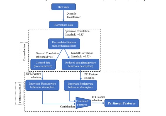
To select the most important features to describe both Ransomware and Benignware behaviours, we follow the process depicted in Figure 1 and described below:

• Apply the PFI technique to the obtained data from the data reduction step, which allows for selecting the most salient features that contribute efficiently to the classification.

• Select the important features regarding Ransomware behaviour, which is done by:
  1. Normalizing the data using a non-linear method,
  2. Reducing the data by combining Spearman and Kendall. Firstly, we use Spearman correlation with a threshold of 0.85 to keep non-redundant features. Then, we usethe Kendall correlation between features and targets with a weak threshold (0.1) to delete noise.
  3. Calculating the importance of features against Ransomware using FICFR.
  4. Selecting features with a FICFR score greater than a fixed threshold (0.1 fixed after experimentation).

Figure 1. feature selection process

3- Combine the first part of features from step 1 with the part of features obtained from step 2. We call the resulting set of features RB important features.
4- Run Ransomware detection using RB important features and track the ML algorithm that gives the best performance.
5- Run PFI again on the ML algorithm selected in step 4 with RB important features and select the features that have a PFI score greater than 0. The obtained set of features, which we call RB salient features, are the last and the most important features used to perform Ransomware detection

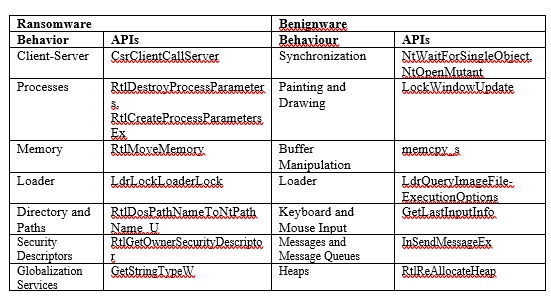
Table 2. List of salient features for Ransomware and Benignware.

According to the results shown in section 4.4.3.3, the best performance reaches 99.81% after K-fold cross-validation (k=10) using MLP with only 16 features (data reduction rate = 99.69%) that describe both Ransomware and Benignware behaviour. Table 2 shows the RB salient features. The last obtained features are the most discriminative system calls. They are related to window drawing and message passing, process loading, memory manipulation, etc. On the other hand, we did not find some API calls indicated in the literature, such as CryptDeriveKey, GetUserName, socket, etc. This is likely due to the diversity of our dataset. The most relevant features listed by their importance are:

• Ldr Query Image File Execution Options: This API is called only by almost all of Benignware, which makes it a very discriminative feature. It is mainly used to enable debug mode or to modify the default application that opens a specified file type in the Windows registry. Therefore, Ransomware typically does not enable debug mode or modify default applications to run with specific file types.
• Nt Wait For Single Object: Waits are necessary to synchronize states across threads. This API is more commonly called Benignware samples.
• Get Last Input Info: This API is used for idle detection and indicates the need for interaction using the keyboard, mouse, screen, etc. Ransomware typically does not require any interaction with the user, unlike many Benignware applications. Therefore, it is unlikely that Ransomware would use this API
• In Send Message Ex: This API is frequently called by many Benignware applications to check whether the window of the current application is handling a message sent by another thread. This is useful for processing the results of threads and checking their state if they are blocked
• memcpy_s: This API is used to copy a memory block from one location to another. It is frequently called by many Benignware applications as an alternative to the memcpy and memmove APIs.
• Ldr Lock Loader Lock: This API is called by a higher number of Ransomware samples. It attempts to enter the critical section known as the loader lock. Once the lock is acquired, the running process can execute code inside DllMain
• RtlDestroyProcessParameters: This API is used by a higher number of Ransomware samples. It is used to release the memory occupied by the parameters passed to the desired process.
• RtlCreateProcessParametersEx: Used by a larger number of Ransomware and a very small number of Benignware, this can be used in conjunction with other APIs such as NtCreateProcessEx and VirtualAllocEx to initiate and run an altered process for malicious purposes.
• RtlGetOwnerSecurityDescriptor: Called at a higher frequency by almost all Ransomware. It returns a pointer to the security identifier (SID) of the owner. The malicious application determines who can access the securable object and which operations can be performed on this resource.
• LockWindowUpdate: Called by Benignware to control drawing on windows and their children.
• CsrClientCallServer: This is called by almost all Ransomware. It invokes routines from the Client Server Runtime Subsystem (CSRSS), which is primarily responsible for Win32 console handling and GUI shutdown.

4. RESULTS AND DISCUSSION

In this section, we present the process of constructing the dataset and collecting the data. Afterwards, we discuss the impact of selecting different methods and algorithms when building our ransomware detection model. We want to emphasize that k-fold cross-validation with k = 10 is used to evaluate the effectiveness of all the models we have built. Additionally, we will measure the performance based on the accuracy criterion given by the following formula :𝐴𝑐𝑐 =(𝑇𝑃 + 𝑇𝑁)/(𝑇𝑃 + 𝑇𝑁 + 𝐹𝑃 + 𝐹𝑁).

4.1. ML algorithms

During the experimentations, we use 8 ML classification techniques namely Decision tree, Adaboost, MLP, RF, XGB, SVM, Logistic regression, and light GBM. The hyperparameters of used ML algorithms are selected using hyperparameter tuning provided by sci-kit-learn to perform an exhaustive search over specified parameter values for an estimator. For each ML algorithm, we provide the  hyperparameter values to keep a trade-off between its performance and the computational cost as follows:

• Decision tree: the main hyperparameter is Maxdepth, the selected value is 80 when the whole features (5194 features) are processed. However, after data reduction, we don’t specify this hyperparameter since we deal with a dozen of features. This allows the tree to split until all leaves are pure.
• Adaboost: we selected the decision tree as the type of weak learner with a Max depth equal to 60 before data reduction and not specified after. Then, we provide 90 as numbers of theestimator.
• Random forest: the selected value of Max depth is 65 before data reduction and not specified after, 90 estimators, and true for the use of bootstrap to improve the stability of the model.
• XGBoost and Light GBM: we select 45 for Max depthbefore data reduction and not specified after, 100 estimators, and learning rateequal to 0.1 to geta an acceptable generalization ability of the model.
• SVM: we chose the use of linear kernel and the selected value of regularization parameter that equals to 1.2 to get better trade-off between the training and testing errors. Then, we put the hyperparameter ‘shrinking’ to true to speed up the training process.
• Logistic regression: we select L1 for the penalty parameter before data reduction and L2 after to prevent the model from overfitting. Then, we put theinverse regularization strength to 100.0 for weak regularization.
• MLP: we use two hidden layers where the size of the first one is 200 units and the second is 100 units. Then, we select the activation function ‘tanh’, the default Maximum number of iterations (200), and the strength of the L2 regularization term equals 0.00001.

4.2. Construction of dataset

This section presents the details of sample download, their execution, and API call collection.

4.2.1. Collection of Benignware and Ransomware

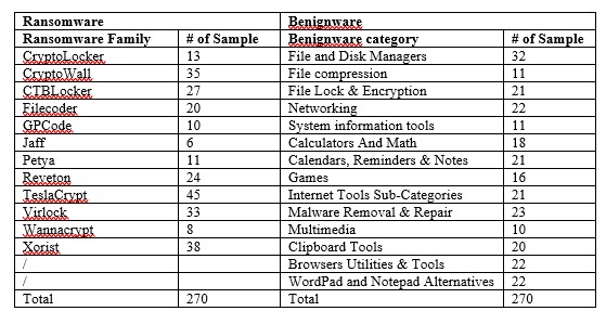
Data collection is a critical operation that requires selecting appropriate samples to include in the study. Firstly, we downloaded 270 samples of both Ransomware and Benignware to create a balanced and diversified dataset. Then, we downloaded ransomware samples from Any.Run, VirusShare, and the Free Automated Malware Analysis Service/Hybrid Analysis dataset. We selected 12 well-known and recent ransomware families, such as WannaCry, CryptoLocker, etc., as depicted in Table 3. On the other hand, we downloaded 270 Benignware samples of various categories from majorgeeks.com and portableapps.com. We selected almost all categories of Benignware to ensure dataset diversity on the one hand and to focus on some kind of application that shares features with ransomware such as encryption, compression, intense access to the file system manager, and network usage. Table 3 shows the categories of Benignware and the families of Ransomware included in our dataset, available in [41].

Table 3. The content of the dataset.

4.2.2. Collection of system calls

To capture system calls, we use a tool called API Monitor. It allows monitoring applications and captures the system calls of running controlled applications, providing useful features such as debugging, parameter decoding, and editing process memory. However, it does not allow automatic exportation of captured system calls to a standard format such as CSV or TXT.

Both Ransomware and Benignware are executed in a virtual machine (guest) having:

• Windows 10, 32-bit system with deactivated firewall and security centre. This allows the known ransomware to be executed and escape the Windows security system.
• 11 GO of data in the system partition and 1.3 GO of data in a separated partition, this data is a set of different file types namely txt, docx, pdf, jpg, png, exe, bat, mp3, and mp4.
• NAT interface. This is useful to connect the guest to the real machine (host).
• INetSim, allows malicious samples to send their requests and to give them the impression that the machine is connected to a real Internet.
• API monitor to capture API calls.

We create an instance of a stable version of the guest machine, and then we run each sample of both ransomware and benign ware separately in a clean session reinitialized behind every execution. Thus, we clean the system from any damages and modifications caused by ransomware to ensure that the next execution occurs in similar conditions. Moreover, we manually run each benign ware file, whether it is portable or installable, to collect its system calls. Once executed, we perform some of its capabilities according to its category, such as cloning a disk or compressing some files. This allows us to capture the APIs called while benign applications process data. Additionally, all types of system calls are collected, including those referenced for data access and storage, graphics and gaming, Component Object Model, etc. Therefore, for each sample, we collect tens of thousands to millions of system calls. The captured system calls for both benignware and ransomware are reported in a global CSV file that consists of API designations as columns and the number of their calls in rows. Finally, we obtained a matrix of 5194 columns/features and 540 rows, which compose the raw data of our dataset.

4.3. Data Normalization

4.3.1. The effect of normalization on the shape of the dataset and the performances

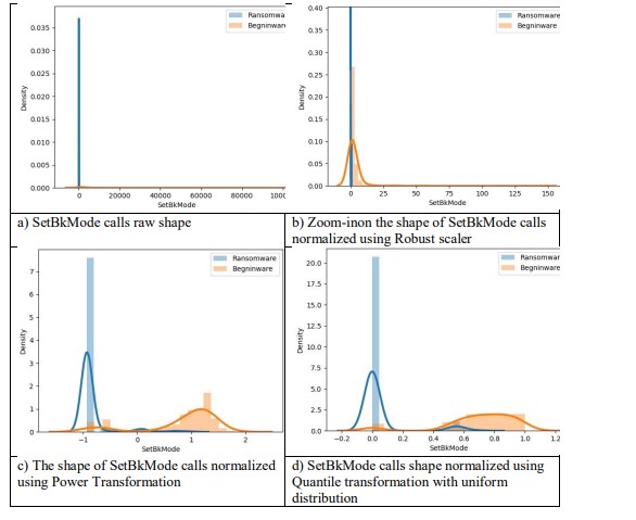
In this experimentation, we demonstrate that the choice of an appropriate normalization method acts on the shape of data and makes them more meaningful. Figure 2 plots the shape of a feature namely “SetBkMode” before and after its normalization. On the X-axis is placed the number of SetBkMode calls, where the Y-axis is the density of calls performed by both Ransomware and Benignware samples. The analyzed normalization techniques are robust scaler, power transformation using “yeo-johnson”, and Quantile transformation with uniform distribution. In the case of linear normalization, the shape of transformed data is the same compared to the original one except for the variation of the range. However, the results of non-linear methods shown in Figures2(c,d) look more meaningful against the distribution of calls for both malware and Benignware. In the case of normalized data using Quantile transformation with uniform distribution, almost all ransomware API calls belong to the range [0, 0.6], whereas almost all of the Benignware API calls belong to the range [0.4, 1] which makes it more likely to distinguish between ransomware and Benignware behaviours.

4.3.2. The effect of normalization on the performances of models

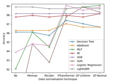
We experiment to show the variation of model performances using different normalization methods. We use both linear normalization methods, namely min-max and Clipping (Robust Scaler with quantile range=(25-75)), and non-linear methods, namely Power Transformer with Yeo-Johnson and Quantile Transformer with both uniform and Gaussian distribution. However, before building the ML models, we reduce the data using Spearman correlation. Firstly, we eliminate features with a correlation threshold of 0.85. Then, we eliminate features with a correlation below 0.48 to the target. We fixed these correlation thresholds after several tests to get the maximum model performance. Figure 3 shows that the accuracies obtained with SVM, MLP, and Logistic regression are notably improved with non-linear normalization methods. Moreover, the highest performance (99.07%) is achieved with MLP and Logistic regression using Power Transformer and Quantile Transformer (normal distribution). However, linear normalization techniques have little or no effect on the performance of Decision Tree, AdaBoost, Random Forest, XGB, and LightGBM. This is due to the presence of outliers in our dataset.

Figure 2. The shape of the API calls of SetBkMode before and after its normalization using various schemes.

Figure 3. The effect of data normalization on the performances of ML models.

Therefore, the use of MLP in addition to linear ML classification algorithms such as SVM and Logistic regression should be applied to non-linearly normalized data. On the other hand, tree-based ML algorithms such as Random Forest, XGB, and LightGBM are not affected by data normalization. Thus, we continue to use non-linear normalization techniques for the remainder of the study.

4.4. Dimensionality Reduction

4.4.1. The selection of Dimensionality reduction technique

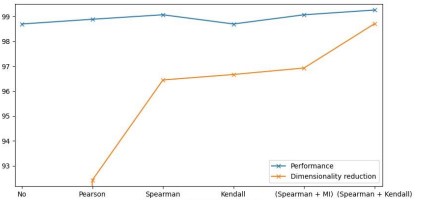
The objective of this section is to identify the most suitable dimensionality reduction technique that can assist ML models in achieving optimal performance. Figure 4 demonstrates that the highest level of data reduction and best performance is achieved by combining the Spearman and Kendall correlation methods. The experiment involved filtering out correlated features and retaining the most relevant feature with respect to the target. Table 4 outlines the dimensionality reduction techniques used in this study, along with their associated thresholds. To eliminate redundant data, we group the correlated features and retain only one feature item from each group, using a fixed threshold (thresh1). The threshold thresh1 is selected based on multiple iterations, and we use the value that yields the best model performance. We note that we could not use the Kendall correlation due to the high number of features and its high computational complexity (O(n^2)), compared to the O(n log n) complexity of the Spearman correlation.

Table 4. Applied correlation score for dimensionality reduction experimentation.

Next, we aim  to remove the features that do not correlate with the target. To achieve this, we define a second threshold score (thresh2). As per Table 4, the best performance of 99.26% is achieved by MLP using a dimensionality reduction technique that combines Spearman and Kendall correlations. After applying the correlation-based feature selection, the number of remaining features is 67, which corresponds to only 1.29% of the raw data.

Figure 4. The best model performances after the application of dimensionality reduction.

4.4.2. ML classification algorithms VS dimensionalityreduction techniques

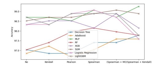
Figure 5 illustrates that the choice of dimensionality reduction technique influences the performance of the built ML models. The highest performances are obtained by MLP using the combination of Spearman and Kendall correlations. However, Adaboost and RF are the most affected by data reduction, in contrast to MLP and SVM

Figure 5. The performances of the ML models were obtained with various data reduction techniques.

Furthermore, the results show that the lowest performances are obtained with Pearson correlation. This is because the measure of linear correlation is not necessarily relevant compared to Spearman and Kendall, which measure the monotonic relationship. Therefore, using Pearson correlation loses some pertinent features when dealing with the target from one side and does not perfectly remove redundant features when measuring linear correlation from the other side. Additionally, we obtained good performances using either Spearman or its combination with MI. However, we cannot favour one over the other except concerning dimensionality reduction, which shows better results using the combination of Spearman and MI. Therefore, we conclude that the use of MI outperforms the dimensionality reduction techniques that rely on Spearman and Pearson correlation. It measures the gained knowledge from features, even if they are not correlated, by calculating the distance between their probability distributions.

On the other hand, we obtain the highest performances when replacing MI with Kendall correlation to measure the relationship between uncorrelated features and the target. This means that Kendall is more efficient and robust, as mentioned in the literature [42]. It uses Kendall tau, which is based on the concordant and discordant pairs to describe non-linear relationships, which are more efficient compared to Spearman rho. In contrast, the use of Kendall correlation affects the computing time and the use of the CPU due to its complexity O(n^2). However, although the best performances were obtained by MLP with 1.29% of data using the combination of Spearman and Kendall, we find that better performances were obtained using almost all ML classification algorithms with either Spearman or its combination with MI on 3.06% of data

4.4.3. Feature selection

In this section, we evaluate the obtained features from the dimensionality reduction, from the FICFR technique, and finally from the combination of PFI and FICFR.

4.4.3.1. The evaluation of obtained features from dimensionality reduction

After reducing the data, we were left with 67 highly correlated features with the target vector. However, upon further analysis, we discovered that these features only describe Benignware behaviours since they were frequently called by almost all of their samples, in contrast to Ransomware. Additionally, we found that 51% of these features were related to Windows Application UI Development and Graphics API. Therefore, we refined the features by applying the PFI technique. Table 5 shows the PFI score assigned to each feature using the MLP algorithm. We only maintained features with positive PFI scores

Table 5. PFI score of important features.

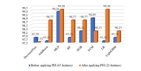
Next, we compared the performance obtained with the resulting features from dimensionality reduction before and after feature selection using the PFI technique. Figure 6 shows that the performance obtained after using feature selection based on PFI outperformed the previous results obtained with reduced data. The maximum performance reached 99.38% using MLP and logistic regression.

Figure 6. performance improvement after feature selection using PFI.

4.4.3.2. Evaluation of features obtained with FICFR technique

As seen in the previous section, the 21 important features are related to the Benignware applications. Thus, we apply feature selection using FICFR to obtain descriptors for Ransomware behaviour. FICFR is applied on normalized, non-redundant, and cleaned data. Data normalization is carried out using a Quantile transformer scheme, redundant data is removed by applying Spearman correlation between features, and finally, noisy data is eliminated by applying the Kendall correlation between features and target vector. The threshold of the Kendall method is slight (0.1) compared to the use of the same correlation technique for dimensionality reduction. This choice is justified by the need to filter out noisy data and retain any feature that can provide additional information regarding Ransomware behaviour. The noisy data, in this case, refers to features that do not have any correlation with the target vector, including the APIs called with the same frequency by both Ransomware and Benignware from one side, and called by few samples whether they are Ransomware or Benignware from the other side. Therefore, applying FICFR allows the selection of highly relevant and frequently called features by Ransomware

4.4.3.3. Combination of Ransomware and Benignware best descriptors

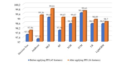
In this experiment, we combined the important features selected by PFI (21 features) with those obtained by FICFR (24 features). As a result, we observed a slight performance improvement and achieved a new record of 99.44% using SVM. Once the features were combined, we ran the PFI selection method again to select the most relevant features. The results showed a new performance record of 99.81% and 99.66% by MLP and SVM respectively after performing Kfold cross-validation (k=10).

Figure 7. Performance improvement after combining FICFR features and selection using PFI.

Table 6. Performance measurements using the set of the pertinent features.

Additionally, we obtained a significant improvement in performance with almost all ML methods using only 16 out of 45 features that had a PFI score greater than 0. Figure 7 illustrates the performances obtained with the combined features before and after the selection using the PFI technique. In addition, table 6 depicts the obtained performance measurements for the different ML algorithms applied  the set of the pertinent features.

Figure 8. Interpretable representation of sample classification using LIME.

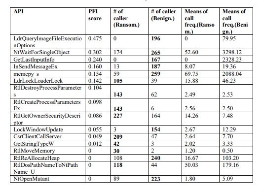
Table 7. The statistics of the pertinent feature.

To visualize the explanations and contribution of each feature in the classification, we use Local Interpretable Model-agnostic Explanations (LIME). Figures 8a and 8b visualize the decision explanations for a Ransomware and Benignware sample respectively. Indeed, the features with a high PFI score are the most influential in the classification. Table 7 shows the statistics of the pertinent features, their PFI score, call frequency, and the number of callers whether they are Ransomware or Benignware.

The pertinent features described in Table 7 are the most discriminative APIs. However, the features with a PFI score of zero for MLP are still useful for other ML algorithms. If we remove them, we still achieve an accuracy of 99.81% with MLP, but we note a decrease of nearly 0.1% for the other models built with the other ML algorithms.

However, the accuracy achieved with our proposed method surpasses that of the state-of-the-art [10, 34, 39, 40]. This can be attributed to our model’s ability to process only the most relevant features, resulting in improved performance and reduced computational costs.

5. CONCLUSION

In this study, we began with the idea that we could differentiate between Ransomware and Benignware based on their behavior regarding activities such as file renaming and encryption. However, these behaviours could also be performed by simple tools for tasks such as file batch renaming, partition management, and file encryption. As a result, we arrived at the actual discriminative features related to the process and thread levels, such as synchronization, the ability to use the Windows registry, debug mode, loader lock, CSRSS server, etc.

To achieve our study, we built a dataset from scratch, collecting Ransomware samples from well-known malware collections, as well as various types of Benignware such as file manipulation and networking tools. Once we prepared our dataset, we normalized the data using a non-linear method and reduced the dimensionality by combining Spearman and Kendall correlation techniques. However, the obtained features only described Benignware behaviour, which led us to introduce a new feature selection technique called FICFR. This technique selects Ransomware features based on their frequency and the number of samples referencing them.

Finally, we built machine learning models using eight different algorithms and achieved impressive performance with 99.81% accuracy using MLP and 99.63% using SVM, with only 16 features.

However, there were some limitations noted during data collection, data reduction, and validation of the ML models, which are:

• Collecting System calls from Ransomware was difficult most of the time due to the absence of the C&C server. We simulated its existence but not its commands.
• The complexity of the calculations performed by the data reduction methods to calculate the correlation between a thousand features.
• The feature selection methods always converge towards choosing those that are related to the execution of benignware, which led us to propose FICFR to select the relevant features from each class.

As feature works we perform the following perspectives:

• Grow up our dataset to include a higher number of Ransomware
• Createan ML-based module to detect zero-day Ransomware attacks which can be used independently or integrated into an anti-virus.
• We turning toward Dynamic Neural Networks since we get the best performance using MLP which is one kind of neural network from one side, and because we believe that there will exist other Ransomware families that we need to include in our study from the other side.

  CONFLICTS OF INTEREST

  The authors declare no conflict of interest.

  ACKNOWLEDGEMENTS

  We would like to express our gratitude to the anonymous reviewers for their insightful comments and suggestions that greatly improved the quality of this manuscript. We also acknowledge the contributions of our colleagues who provided valuable feedback and support throughout the project. Lastly, we would like to thank our families for their patience and understanding during the writing process.

REFERENCES

[1] T. (2022, May 11). 22 Shocking Ransomware Statistics for Cybersecurity in 2021. Safe At Last. https://safeatlast.co/blog/ransomware-statistics/
[2] Maurya, A. K., Kumar, N., Agrawal, A., & Khan, R. (2018). Ransomware: evolution, target and safety measures. International Journal of Computer Sciences and Engineering, 6(1), 80-85.
[3] Ransomware as a Service: 8 Known RaaS Threats. (2021, March 23). Infosec Resources. https://resources.infosecinstitute.com/topic/ransomware-as-a-service-8-known-raas-threats/
[4] Xu, B., Li, Y., & Yu, X. (2020, October). Malware Detection Based on Static and Dynamic Features Analysis. In International Conference on Machine Learning for Cyber Security (pp. 111-124). Springer, Cham.
[5] Hsiao, S. C., & Kao, D. Y. (2018, February). The static analysis of WannaCry ransomware. In 2018 20th International Conference on Advanced Communication Technology (ICACT) (pp. 153-158). IEEE.
[6] Carlin, D., O’Kane, P., &Sezer, S. (2018, June). Dynamic Opcode Analysis of Ransomware. In 2018 International Conference on Cyber Security and Protection of Digital Services (Cyber Security) (pp. 1-4). IEEE.
[7] Carlin, D., O’Kane, P., &Sezer, S. (2017). Dynamic analysis of malware using run-time opcodes. In Data analytics and decision support for cybersecurity (pp. 99-125). Springer, Cham.
[8] Hăjmăȿan, G., Mondoc, A., &Creț, O. (2019, September). Bytecode Heuristic Signatures for Detecting Malware Behavior. In 2019 Conference on Next Generation Computing Applications (NextComp) (pp. 1-6). IEEE.
[9] Mercaldo, F., Nardone, V., Santone, A., &Visaggio, C. A. (2016, June). Ransomware steals your phone. formal methods rescue it. In International Conference on Formal Techniques for Distributed Objects, Components, and Systems (pp. 212-221). Springer, Cham.
[10] Bae, S. I., Lee, G. B., &Im, E. G. (2020). Ransomware detection using machine learning algorithms. Concurrency and Computation: Practice and Experience, 32(18), e5422.
[11] Arabo, A., Dijoux, R., Poulain, T., & Chevalier, G. (2020). Detecting Ransomware Using Process Behavior Analysis. Procedia Computer Science, 168, 289-296.
[12] Pektaş, A. (2018). Mining patterns of sequential malicious APIs to detect malware. International Journal of Network Security & Its Applications (IJNSA) Vol, 10.
[13] Cabaj, K., Gregorczyk, M., &Mazurczyk, W. (2018). Software-defined networking-based crypto ransomware detection using HTTP traffic characteristics. Computers & Electrical Engineering, 66, 353-368.
[14] Wan, Y.-L., Chang, J.-C., Chen, R.-J., & Wang, S.-J. (2018). Feature-Selection-Based Ransomware Detection with Machine Learning of Data Analysis. 2018 3rd International Conference on Computer and Communication Systems (ICS), 85 88. https://doi.org/10.1109/CCOMS.2018.8463300
[15] Huynh, T. T., & Nguyen, T. H. (2021). On the performance of intrusion detection systems with hidden multilayer neural network using DSD training. International Journal of Computer Networks & Communications (IJCNC), 117-137.
[16] Aurangzeb, S., Rais, R. N. B., Aleem, M., Islam, M. A., & Iqbal, M. A. (2021). On the classification of Microsoft-Windows ransomware using hardware profile. PeerJ Computer Science, 7, e361. https://doi.org/10.7717/peerj-cs.361
[17] Sayadi, H., Makrani, H. M., PudukotaiDinakarrao, S. M., Mohsenin, T., Sasan, A., Rafatirad, S., & Homayoun, H. (2019). 2SMaRT: A Two-Stage Machine Learning-Based Approach for Run-Time Specialized Hardware-Assisted Malware Detection. 2019 Design, Automation & Test in Europe Conference & Exhibition (DATE), 728 733. https://doi.org/10.23919/DATE.2019.8715080
[18] Lu, T., Zhang, L., Wang, S., & Gong, Q. (2017, December). Ransomware detection isbased on V-detector negative selection algorithm. In 2017 International Conference on Security, Pattern Analysis, and Cybernetics (SPAC) (pp. 531-536). IEEE.
[19] Khammas, B. M. (2020). Ransomware Detection using Random Forest Technique. ICT Express, 6(4), 325 331. https://doi.org/10.1016/j.icte.2020.11.001
[20] Homayoun, S., Dehghantanha, A., Ahmadzadeh, M., Hashemi, S., &Khayami, R. (2020). Know Abnormal, Find Evil : Frequent Pattern Mining for Ransomware Threat Hunting and Intelligence. IEEE Transactions on Emerging Topics in Computing, 8(2), 341 351. https://doi.org/10.1109/TETC.2017.2756908
[21] Euh, S., Lee, H., Kim, D., & Hwang, D. (2020). Comparative Analysis of Low-Dimensional Features and Tree-Based Ensembles for Malware Detection Systems. IEEE Access, 8, 76796 76808. https://doi.org/10.1109/ACCESS.2020.2986014
[22] Al-Akhras, M., Alawairdhi, M., Alkoudari, A., &Atawneh, S. (2020). Using machine learning to build a classification model for iot networks to detect attack signatures. Int. J. Comput. Netw. Commun.(IJCNC), 12, 99-116.
[23] Sultan, M. T., Sayed, H. E., & Khan, M. A. (2023). An Intrusion Detection Mechanism for MANETs Based on Deep Learning Artificial Neural Networks (ANNs). arXiv preprint arXiv:2303.08248.
[24] Roy, K. C., & Chen, Q. (2021). DeepRan : Attention-based BiLSTM and CRF for Ransomware Early Detection and Classification. Information Systems Frontiers, 23(2), 299 315. https://doi.org/10.1007/s10796-020-10017-4
[25] Gaur, K., Kumar, N., Handa, A., & Shukla, S. K. (2021). Static Ransomware Analysis Using Machine Learning and Deep Learning Models. In M. Anbar, N. Abdullah, & S. Manickam (Éds.), Advances in Cyber Security (p. 450 467). Springer. https://doi.org/10.1007/978-981-33-6835-4_30
[26] Takeuchi, Y., Sakai, K., & Fukumoto, S. (2018). Detecting Ransomware using Support Vector Machines. Proceedings of the 47th International Conference on Parallel Processing Companion, 1 6. https://doi.org/10.1145/3229710.3229726
[27] Adamu, U., & Awan, I. (2019). Ransomware Prediction Using Supervised Learning Algorithms. 2019 7th International Conference on Future Internet of Things and Cloud (FiCloud), 57 63. https://doi.org/10.1109/FiCloud.2019.00016
[28] Interactive Online Malware Analysis Sandbox—ANY.RUN. (s. d.). (2022, June 13). https://app.any.run/
[29] VirusShare.com. (s. d.). (2022, June 13). https://virusshare.com/
[30] VirusTotal. (s. d.). (2022, June 13). https://www.virustotal.com/gui/
[31] Ytisf/theZoo [Python]. (2022, June 27). https://github.com/ytisf/theZoo/
[32] MAEC – Malware Attribute Enumeration and Characterization | MAEC Project Documentation. (s. d.). (2022, June 25). https://maecproject.github.io/
[33] Azeez, N. A., Odufuwa, O. E., Misra, S., Oluranti, J., &Damaševičius, R. (2021). Windows PE Malware Detection Using Ensemble Learning. Informatics, 8(1), 10. https://doi.org/10.3390/informatics8010010
[34] Poudyal, S., Subedi, K. P., & Dasgupta, D. (2018, November). A framework for analyzing ransomware using machine learning. In 2018 IEEE Symposium Series on Computational Intelligence (SSCI) (pp. 1692-1699). IEEE.
[35] Catak, F. O., Yazı, A. F., Elezaj, O., & Ahmed, J. (2020). Deep learning based Sequential model for malware analysis using Windows exe API Calls. PeerJ Computer Science, 6, e285. https://doi.org/10.7717/peerj-cs.285
[36] Catak, F. O. (2021). Ocatak/malware_api_class [Python]. (2022, June 27). https://github.com/ocatak/malware_api_class
[37] Hasan, M. A. M., Nasser, M., Ahmad, S., &Molla, K. I. (2016). Feature Selection for Intrusion Detection Using Random Forest. Journal of Information Security, 7(3), 129 140. https://doi.org/10.4236/jis.2016.73009
[38] Priya, R. H., & Bhagavan, K. (2019). Anti –Reverse Engineering Techniques Employed by Malware. 8(6), 5.
[39] Chen, Z. G., Kang, H. S., Yin, S. N., & Kim, S. R. (2017, September). Automatic ransomware detection and analysis based on dynamic API call flow graph. In Proceedings of the International Conference on Research in Adaptive and Convergent Systems (pp. 196-201).
[40] Shaukat, S. K., & Ribeiro, V. J. (2018, January). RansomWall: A layered defence system against cryptographic ransomware attacks using machine learning. In 2018 10th International Conference on Communication Systems & Networks (COMSNETS) (pp. 356-363). IEEE.
[41] Dib, A., Ghazi, S., &Mendjel, M. S. M. (2022), “Ransomware/Benignware System Calls”, Mendeley Data, V1, doi: 10.17632/kbt8xt3678.1
[42] Newson, R. (2002). Parameters behind “Nonparametric” Statistics : Kendall’s tau, Somers’ D and Median Differences. The Stata Journal: Promoting Communications on Statistics and Stata, 2(1), 45 64. https://doi.org/10.1177/1536867X0200200103
[43] Hampton, N., Baig, Z., &Zeadally, S. (2018). Ransomware behavioural analysis on Windows platforms. Journal of information security and applications, 40, 44-51.