IJCNC 01

PERFORMANCE EVALUATION OF ERGR-EMHC ROUTING PROTOCOL USING LSWTS AND 3DUL
LOCALIZATION SCHEMES IN UWSNS

Faiza Al-Salti1 , N. Alzeidi2 , Khaled Day2 , Abderezak Touzene2

1Department of Informatics and Cyber Security, Sultan Qaboos Comprehensive Cancer
Care and Research Centre, Oman
2Department of Computer Science, Sultan Qaboos University, Oman

ABSTRACT
This paper studies the impact of different localization schemes on the performance of location-based routing for UWSNs. Particularly, LSWTS and 3DUL localization schemes available in the literature are used to study their effects on the performance of the ERGR-EMHC routing protocol. First, we assess the performance of two localization schemes by measuring their localization coverage, accuracy, control packets overhead, and required localization time. We then study the performance of the ERGR-EMHC protocol using location information provided by the selected localization schemes. The results are compared with the performance of the routing protocol when using exact nodes’ locations. The obtained results show that LSWTS outperforms 3DUL in terms of localization accuracy by 83% and localization overhead by 70%. In addition, the results indicate that the localization error has a significant impact on he performance of the routing protocol. For instance, ERGR-EMHC with LSWTS is better in delivering data packets by an average of 175% compared to 3DUL

KEYWORDS
Underwater wireless sensor networks (UWSNs), localization, ranging localization methods, localization error, location-based routing

1. INTRODUCTION
Location-based routing protocols are widely used in Underwater Wireless Sensor Networks (UWSNs). They do not require the dissemination of route discovery packets; instead, they use location information of neighboring nodes to forward packets [1]. Consequently, less overhead and high scalability can be achieved with such schemes. However, the nature of the underwater environment induces several challenges in localizing nodes. Examples of these challenges are [2], [3](iii) GPS does not work well underwater due to the high attenuation of radio waves in such environments. Thus, several localization schemes have been developed specifically for UWSNs to address these issues (e.g.,[4], [5], [6], [7],[8],[9]). Nevertheless, the developed routing protocols have been assessed with the assumption that all nodes can obtain their locations accurately (e.g.,[10], [11], [12], [13], [14]. This assumption might not be valid as some nodes might get inaccurate locations as well as some others might fail to get their locations completely. This is due to the errors in distance estimation and to the inability of some nodes to receive sufficient information required for location estimation.

Various research papers found that localization inaccuracies worsen the performance of locationbased routing protocols in WSNs. B. Peng et al.[15] and M. Kadi et al.[16] have studied the impact of localization error on energy consumption. They have proposed error models and they have verified the need to cope with the localization inaccuracies while designing location-basedrouting protocols. The authors in [15] have further proposed a routing protocol called Least Expected Distance (LED) protocol, which selects the next forwarder that optimizes energy consumption in the presence of location errors. Shah et al.[17] have analyzed the impact of location errors on energy consumption and packet delivery ratio (PDR) of location-based routing schemes that use greedy forwarding mechanisms. Their results have shown that the performance degrades significantly with location errors of more than 20% of the transmission range. Son et al.[18] have studied the impact of location errors resulting from node mobility on energy consumption and PDR. They have proposed two mobility-prediction algorithms to mitigate the effects of location errors. Their simulation results have revealed an improvement of about 27% in PDR and 37% in energy consumption.

To the best of our knowledge, however, no work has studied the impact of localization schemes on the performance of location-based routing in UWSNs. Therefore, this paper aims to analyze the impact of different localization schemes on the performance of the Efficient and Reliable Grid-based Routing by Exploiting Minimum Hop Count(ERGR-EMHC) routing protocol proposed in [14]. The obtained results are expected to give some insights on how to generalize the impact on other location-based routing protocols in UWSNs. More precisely, the contributions of this paper are to:

• Compare the performance of two localization schemes proposed for UWSNs, namely the Localization Scheme Without Time Synchronization (LSWTS) [5] and the ThreeDimensional Underwater Localization (3DUL) [6]. We assess their performance, in terms of localization coverage, accuracy, control messages overhead, and required time. The 3DUL and LSWTS localization schemes are selected for the following reasons. First, time synchronization between nodes which is one of the most challenges in UWSNs is not required. Second, there is a detailed description of the protocols sufficient for implementing them. Third, the two schemes use two different and commonly used methods for distance measurements (i.e., the dive and raise method and the projection method). Furthermore, the 3DUL is enhanced by adding an error threshold as a confidence value and assesses the associated performance gains.
• Study the performance of the ERGR-EMHC [14]protocol using location information provided by 3DUL, LSWTS and enhanced 3DUL. The results are compared with the performance of the protocol when using the exact locations obtained from the simulator(we called it built-in localization method).
• The paper basically aims to answer the following research questions:
• How the performance (in terms of localization coverage, localization error, localization time, and localization overhead)of the 3DUL and LSWTS can be improved by adding error threshold?
• What is the performance of ERGR-EMHC when using 3DUL, LSWTS and enhanced 3DUL compared to using the built-in localization scheme?

The rest of the paper is organized as follows. Section 2 presents a brief overview of the ERGREMHC routing protocol. It also provides a summary of localization devices, different classifications of localization schemes as well as an overview of the 3DUL, LSWTS and enhanced 3DUL localization schemes. Section 3 compares the performance of the selected localization schemes against each other according to some specific metrics. The impact of these schemes on the performance of the ERGR-EMHC routing protocol is investigated in section 4. Finally, section 5 concludes the paper.

2. PRELIMINARIES
2.1. Overview of the ERGR-EMHC Protocol
The ERGR-EMHC [14] is a grid-based routing protocol, in which the network is viewed as a collection of cells forming a 3D grid, and the forwarding is performed in a cell-by-cell manner until the packet reaches the sink nodes at the surface level. The protocol classifies the neighboring cells into two groups according to their minimum hop count to the closest sink cell. Furthermore, it adopts an election algorithm to elect a cell-head node in each cell. The election is based on the nodes’ remaining energy and the distances to the center of the nodes’ hosting cells. Data packets are forwarded using selected nodes. The number of hops of each packet can be dynamically selected by the source nodes. To solve the void problem, the protocol uses negative acknowledgments and retransmissions. Refer to [14] for more details on this protocol.

• 2.2. Localization Devices
  To implement a localization scheme in UWSNs, four different types of nodes can be used. Surface buoys: These devices placed on the water surface and know their locations most likely through GPS receivers.
• Underwater anchor nodes: nodes with known locations deployed underwater. These devices along with anchor devices are used to localize other nodes
• Ordinary nodes: nodes deployed underwater to be located.
• Reference nodes: nodes with known location. A reference node could be a surface buoy, an anchor node or an ordinary node after being located and they are used to localize other nodes with unknown locations.

2.3. Classification of Localization Schemes
Generally, the localization schemes can be classified based on three criteria as follows:

• Range measurement: the localization schemes can be classified as range-based, rangefree and hybrid. Range-based schemes (e.g., LSWTS [5], DNR [19], 3DUL [6], SLMP [7]) use range information to estimate nodes’ location. Range-free schemes (e.g., ALS [20], 3D-MALS [8]), in contrast, are affected by nodes’ connectivity. Hybrid schemes (e.g., TP-TSFLA [9]) combine both range-based and range-free techniques to estimate locations coordinates.
• Multi/single stage: as the localization process progresses, ordinary nodes can determine their locations. These nodes can be used as reference nodes that help localize other nodes, which in turn improves the localization time and coverage. Such schemes are called multi-stage schemes (e.g., 3DUL [6], SLMP [7]). However, localization errors in such schemes accumulate in each stage due to the possible errors that occur in the distance estimation. On the other hand, some of the localization schemes prevent such nods from helping in localizing other nodes. Such schemes are called single-stage localization schemes (e.g., LSWTS [5], DNR [19], ALS [20]). The main weaknesses of such schemes are the high delay, and the need for more anchor nodes to achieve high coverage.
• Active/silent localization: In active localization schemes (e.g., 3DUL [6], ALS [20]), ordinary nodes also exchange packets to complete the localization process. In silent localization schemes (e.g., LSWTS [5], DNR [19], SLMP [7]), on the contrary, ordinary nodes passively listen to the localization packets transmitted by anchor nodes

2.4. The LSWTS Localization Scheme
LSWTS [5] is a range-based, single-stage and silent localization scheme. It assumes the availability of two types of devices; mobile beacons and static sensor nodes. Beacon nodes dive and rise vertically at constant speed, v, known by every sensor node. They gather their location coordinates from GPS when rising at the surface. While diving, they broadcast localization messages at fixed intervals. A sensor node upon receiving two messages from a beacon node at different depths (say z1 and z2) calculates its distance d to that beacon. The calculation depends on the depth of the beacon relative to the depth of the sensor node (say z3), and there are three different cases as given in Table 1, where c is the speed of the sound underwater (assumed  constant and equal to 1500 m/s). After computing the distance from three beacon nodes, the sensor node estimates its position using trilateration (refer to [3] for a more detailed explanation of this method).

Table 1. The three different cases of distance measurement in LSWTS

2.5. The 3DUL Localization Scheme

3DUL [6] is a range-based, multi-stage and active localization scheme. It assumes the availability of two types of nodes; beacon nodes and sensor nodes. It consists of a ranging phase and a projection phase. During the ranging phase, the surface buoys broadcast anchor range packets. When an ordinary node receives three such packets from three different beacon nodes, it broadcasts a ranging packet to initiate distance measurement and records the time of sending (say T1). The beacon node upon receiving a ranging packet replies with an acknowledgment packet containing the reception time (say T2) and sending time (say T3). When the ordinary n ode receives this packet (say at T4), it calculates the propagation time tprop as follows:

This two-way message exchange is illustrated in Figure 1. The process is followed by the estimation of the distance between the beacon nodes and the sensor node as given in (5). During the projection phase, the node calculates the distance after projection (𝑑′ ) as given in [3]. If the ordinary node calculates the distance to at least three reference nodes, it estimates its position using trilateration. Then, the node becomes a reference node and helps in locating the remaining ordinary nodes.

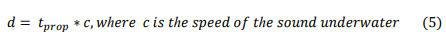
Figure 1. Two-way message exchange in 3DUL scheme

2.6. The enhanced 3DUL Localization Scheme
To reduce the localization error of the multi-stage localization scheme (3DUL scheme in our case), we assess a new version of 3DUL (called E-3DUL) by adding an error threshold. This error threshold is used by ordinary nodes to decide whether the estimation of the location is within an acceptable error range or not. A similar version for LSWTS scheme (called E-LSWTS) is also added to test whether the performance of the single-stage schemes is affected by this error threshold or not.

3. PERFORMANCE COMPARISON OF 3DUL, E-3DUL, LSWTS AND ELSWTS SCHEMES
3.1. Simulation Setup
We have implemented 3DUL, LSWTS, E-3DUL and E-LSWTS localization schemes in the Aqua-sim simulator. A. M. Abu-Mahfouz et al.[21] proposed an extension to NS2 simulator to evaluate localization schemes. We have installed the extension in the Aqua-sim and then implemented the four localization schemes. We have also implemented the mobility model used by LSWTS. The mobility model used to simulate the vertical movement of beacon nodes in LSWTS and E-LSWTS. Sensor nodes are deployed randomly in a 3D area of size (3*3*3) km3 The performance of the localization schemes has been evaluated by assessing the following performance metrics [22][6][23][7][24]:

•  Localization Coverage (CL): It measures the ratio of the localized nodes by a localization scheme to all sensor nodes. Formally, it can be represented as:

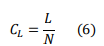
Where L denotes the number of localized nodes and N represents the number of sensor nodes in the network.

• Normalized Localization Error (EL): The error of the localization scheme is measured by calculating the average distance between the estimated location and the true location. The value is then normalized to the transmission range (R)of the nodes. Formally, it can be expressed as follows:

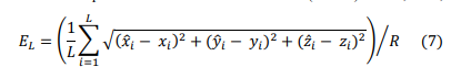
Where (𝑥̂𝑖 , 𝑦̂𝑖 , 𝑧̂𝑖) is the estimated location of the node i, (𝑥𝑖 , 𝑦𝑖 , 𝑧𝑖 ) is the true location of the node i and L is the number of localized nodes. Recall that 3DUL and LSWTS use pressure sensors to obtain the depth of the node and the estimation is performed only for xydimensions. Thus, the term 𝑧̂𝑖 − 𝑧𝑖 in equation 7 has no effect (i.e., has zero value) and can be removed

•  Localization Overhead (OL):It can be defined as the average number of localization packets sent by all nodes over the total number of localized nodes. Formally, it can be represented as:

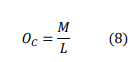
Where M is the total number of localization packets and L is the number of localized nodes.

• Localization Time (TL):It is the time required to localize the L (localized) nodes. Obviously, higher localization coverage, lower localization error, lower communication overhead and lower localization time indicate better performance of the corresponding localization scheme. These performance metrics are investigated by varying the following parameters:
• Number of Beacon Nodes: The impact of the number of beacon nodes is assessed by varying its values from 2.5% to 7.5% of the total number of ordinary nodes (200 sensor nodes). Nodes are randomly deployed in the area. The transmission range of the nodes is set to 1500 m.
• Transmission Range: The impact of the transmission range is investigated by setting its values to 500 m, 1000 m and 1500 m. A total of 10 beacon nodes are used in this set of experiments. Furthermore, 200 sensor nodes are randomly deployed in the environment.

The positions of the beacon nodes are selected according to the multiple sink placement scheme proposed in [25], while the sensor nodes are deployed randomly in the area. An error threshold of 0.98*R, where R is the transmission range is used for the E-3DUL and E-LSWTS. The results of both versions of each scheme, if not otherwise explicitly mentioned, are found the same. 95% confidence intervals are calculated for all collected results. The average of 25 batch runs along with error bars are presented in the figures. Table 2 lists some additional simulation parameters.

Table 2. Additional simulation parameters

Impact of the Number of Beacon Nodes

Figure 2.a demonstrates the impact of the number of beacon nodes on the localization coverage. Generally, the localization coverage increases with the increase in the number of beacon nodes. However, both versions of the 3DUL scheme outperform LSWTS in terms of localization coverage in all scenarios. This is reasonable since 3DUL is a multi-stage scheme in which the number of reference nodes, which can help in localizing other nodes, increases with time. In LSWTS, on the other hand, only beacon nodes act as reference nodes and other nodes remain silent. Therefore, some nodes like those located on the edges are unable to receive a sufficient number of location messages to estimate their locations. As the number of beacons increases from 2.5% to 7.5% of the number of ordinary nodes, the coverage of the 3DUL is maintained at nearly 100%, while the coverage of the LSWTS increases from 40% to 70%. Furthermore, incorporating the error threshold has no impact on the localization coverage of both schemes. Though, the high coverage of 3DUL comes at the cost of high localization error and high localization overhead as shown in figures 2.b and 2.c.

Figure 2.b depicts the relationship between the localization error and the number of beacon nodes. Clearly, LSWTS is more accurate than 3DUL in location estimation over all used number of beacon nodes. This is expected since the reference nodes used for location estimation in LSWTS are only the beacon nodes, which have accurate location information. In 3DUL, on the other hand, localized sensor nodes participate in localizing other nodes; thus, the error in location estimation accumulates with time. With the increase in the percentage of beacon nodes, the localization error of 3DUL and E-3DUL decreases. For example, when the beacon percentage is 2.5%, the localization error of 3DUL and E-3DUL is 1.32 and 0.63, respectively. However, when the beacon percentage increases to 5%, the localization error of the schemes reduces to 1.27 and 0.61, respectively. This can be explained as follows. When the beacon percentage increases, sensor nodes will get to know more beacon nodes and can calculate their positions more accurately. However, the localization error of LSWTS is almost the same over all used beacon percentages. For example, the difference between the localization error at 2.5% and 7.5% is just 0.0015. It is also worth noting that adding an error threshold improves the accuracy of 3DUL. For instance, with 5% beacon nodes, E-3DUL exhibited less than half the localization error exhibited by 3DUL.

Figure 2.c reveals that generally the communication overhead increases with the increase in the number of beacon nodes. Although the number of localized nodes in 3DUL is much higher than LSWTS, LSWTS outperforms 3DUL in terms of localization overhead, which can be justified as follows. In LSWTS, only beacon nodes broadcast localization packets. Other nodes (i.e., other reference nodes and ordinary nodes) remain silent. In 3DUL, however, beacon nodes and ordinary nodes use two-way message exchanges to avoid clock synchronization between them. Thus, the average communication overhead in LSWTS is very small compared to the 3DUL. The E-3DUL exhibits the worst overhead since some ordinary nodes need to run the location estimation more than once to achieve the specified error threshold.

Figure 2.d plots the relationship between the number of beacon nodes and the localization time. We can observe that there is almost no change in the localization time of all localization schemes with the increase in the number of beacon nodes. We can also observe that 3DUL scheme locates nodes much faster than LSWTS scheme. This is due to the fact that 3DUL is a multi-stage localization scheme, whereas LSWTS is a single-stage localization scheme. For example, when the beacon percentage is set to 5%, 3DUL scheme is able to localize 99% of the sensor nodes in 27.6 seconds, while LSWTS needs 964.7 seconds to localize only 63.8% of the total sensor nodes.

Figure 2. Impact of the number of beacon nodes on the (a) localization coverage, (b) localization error (c) localization overhead and (d) localization time

Impact of the Transmission Range

Figure 3.a shows that generally the localization coverage exhibited by the used localization schemes increases with the increase in the transmission range. This can be justified by the fact that as the transmission range increases, the number of isolated nodes and those located on the edges are able to receive a sufficient number of location messages to estimate their locations. However, the increase is of different rate, which can be justified as follows. 3DUL localizes nodes faster than E-3DUL and LSWTS because it is a multi-stage scheme and there is no error threshold. E-3DUL achieves the lowest coverage when the transmission range varies from 500 m to 1000 m because few nodes can obtain their locations with accuracy levels less than the threshold. However, when the transmission range is set to 1500 m, the coverage reaches 99% as nodes can receive more accurate information. Finally, LSWTS depends only on messages from beacon nodes, therefore as the transmission range of these beacons increases, sensor nodes can obtain sufficient number of messages to estimate their locations. Specifically, by increasing the transmission range from 1000 m to 1500 m, the localization coverage increases from 0.82 to 1 for 3DUL, from 0.01 to 0.99 for E-3DUL and from 0.27 to 0.64 for both versions of LSWTS.

Figure 3.b plots the relationship between the transmission rangeand the localization error. Overall, LSWTS outperforms 3DUL in the accuracy of the localization error as it depends only on beacon nodes in locating nodes. These beacon nodes know their locations accurately. In the 3DUL scheme, however, the error in location estimation accumulates with time because the localized sensor nodes participate in locating other nodes. Particularly, when the transmission range is set to 1000 m, LSWTS reduces the localization error by 79% and 94% compared to E- 3DUL and 3DUL, respectively. The 3DUL shows a significant decrease by 37.8% in the localization error with the increase in the transmission range from 1000 to 1500. This can be justified as follows. As the transmission range increases, sensor nodes are able to depend more on accurate information to estimate their locations.

Figure 3.c represents the localization overhead as a function of the transmission range. Generally, all schemes exhibit declines in the localization overhead with the increase in the transmission range due to the increase in the number of localized nodes. With 500 m increase in the transmission range from 1000 m to 1500 m, the 3DUL, E-3DUL and LSWTS show a decline by 28.9%, 62.5% and 56.8%, respectively.

Figure 3.d reveals the localization time as a function of the transmission range. As the transmission range increases, 3DUL schemes locate nodes faster than LSWTS independently of the transmission range. 3DUL and E-3DUL can localize 99% of nodes within 28 seconds, while LSWTS localizes only 64% of the sensor nodes within 965 seconds.

Figure 3. Impact of the transmission range on the (a) localization coverage, (b) localization error, (c) localization overhead and (d) localization time

Discussion

Figures 2 and 3 show that the 3DUL scheme outperforms LSWTS in terms of localization coverage and required localization time. However, this comes at the cost of higher localization error and higher overhead. The localization error of the 3DUL can be reduced by adding an error threshold to prevent ordinary nodes from being localized when the location error is higher than the threshold. It is also worth mentioning that the threshold has almost no effect on the performance of LSWTS. Therefore, the localization error of the multi-stage scheme can be significantly reduced by adding an error threshold.

Furthermore, the results suggest that with 10 beacon nodes and transmission range of 1500 m, 3DUL can localize 100% of the nodes in 23 seconds but at the cost of 1.28 error and 15.22 overhead (i.e., 15.22 localization packets per localized node). With the same percentage of beacon nodes and transmission range, E-3DUL localizes 99% in 27 seconds with 0.61 error and 26.61 overhead. On the other hand, LSWTS localizes only 64% in 965 seconds at the cost of 0.1 error and 1.96 overhead.

4. ERGR-EMHC PERFORMANCE USING 3DUL AND LSWTS

This section investigates the impact of the 3DUL, E-3DUL, LSWTS and E-LSWTS localization schemes on the performance of the ERGR-EMHC protocol. The results are compared against those achieved when using the built-in localization method in the simulator.

Simulation Setup

We used the same simulation setup mentioned in section 3. The experiments are conducted by varying the number of deployed sensor nodes and the number of source nodes generating traffic. Recall that the ERGR-EMHC routing protocol depends on location information to construct the grid and it assumes that all nodes can obtain their locations at any time. However, as noticed in the results above, the 3DUL and LSWTS schemes were not able to achieve 100% coverage in almost all scenarios. Therefore, nodes that fail to get their locations cannot be used as source nodes or as relay nodes. The transmission range of the nodes is set to 1500 m and 10 beacons are used in these experiments. The performance metrics used in this set of experiments are similar to those given in [14], which are as follows:

• Packet Delivery Ratio (PDR): PDR is the ratio of the number of distinct data packets received successfully by the surface base stations (sink nodes) to the total number of created data packets [26].

• Average End-to-End Delay: It is the average time taken by a data packet to arrive to the destination. It is computed from the time the packet is generated until it reachesthe destination. Only data packets that were successfully delivered to the sink nodes are considered.

• Energy Consumption: It is the total sum of transmission energy, reception energy and energy consumed when the sensors are in idle modes.

• Normalized Network Overhead (NNO): The NNO is the ratio of the number of control packets transmitted by the sensor nodes to the number of distinct data packet received by the sink nodes.

These metrics are studied under the effect of varying the following parameters:

• Number of Sensor Nodes: The impact of the number of sensor nodes is assessed by setting the number of sensor nodes to 100, 200, and 300. A total of 10 sensor nodes from the localized nodes are selected randomly as source nodes.

• Traffic Load: The impact of the traffic load is assessed by varying the number of source nodes generating traffic among the values 2.5%, 5% and 7.5% of the total number of sensor nodes which is set to 300 nodes. These source nodes are randomly chosen from the set of localized nodes.

Table 3. Additional simulation parameters

Impact of the Number of Deployed Sensor Nodes

Figure 4.a reveals the relationship between the number of sensor nodes and energy consumption. In general, ERGR-EMHC shows a directly proportional relationship between energy consumption and the number of deployed sensor nodes with all used localization methods. Nevertheless, the protocol consumes less energy with LSWTS, which can be justified as follows. Since LSWTS has the lowest coverage, a smaller number of nodes participate in transmitting and receiving packets compared to the 3DUL and the built-in localization schemes. For instance, when the number of sensor nodes is set to 200, the coverage of LSWTS and 3DUL is 64% and 100%, respectively. Although the coverage of the 3DUL is 100%, ERGR-EMHC consumes less energy with the built-in localization schemes compared to the 3DUL. This is because the localization error of the 3DUL is very high; thus, it leads to inaccurately assigning cell IDs to nodes. This increases the probability of transmission failures of data packets.

The average end-to-end delay is shown as a function of the number of sensor nodes in Figure

4.b. Generally, the figure reveals that ERGR-EMHC exhibits almost similar average end-to-end delay when using the built-in and the LSWTS localization methods. Although the coverage of 3DUL is better than LSWTS, the localization error in 3DUL is the worst. Thus, the increase in the localization error offsets the advantages of higher localization coverage. It is worth mentioning that with 200 sensor nodes, ERGR-EMHC with LSWTS is faster in delivering data packets than 3DUL and E-3DUL by 65% and 50%, respectively.

Figure 4.c shows the impact of the number of deployed sensor nodes on the PDR. Not surprisingly, the PDR increases with the increase in the number of deployed sensor nodes under all localization schemes. This can be justified by the increase in the probability of locating candidate forwarders. As the number of nodes increases, the PDR achieved with LSWTS gets closer to that with the built-in localization method. Furthermore, LSWTS achieves higher PDR than 3DUL. Specifically, when the number of sensor nodes is set to 200, the protocol with the built-in localization method achieves PDR higher than that with LSWTS, E-3DUL and 3DUL by 3.2%, 36.9%, and 75.6%, respectively. This is because the built-in localization method gives 100% accurate location for each sensor node; hence, the obtained CIDs of each node is 100% accurate. Although the number of located nodes with the 3DUL is higher than that of LSWTS, the localization error with 3DUL is higher (hence the PDR with 3DUL is lower).

Figure 4.d shows the effect of the number of sensor nodes on the routing overhead. LSWTS outperforms the other localization methods by exhibiting the lowest routing overhead and 3DUL is the worst. As the number of nodes increases, the routing overhead of 3DUL decreases, and it becomes closer to other methods. This is due to the decrease in the localization error. With 200 sensor nodes, the routing overhead incurred using LSWTS is lower than that using the built-in localization scheme, 3DUL.98 and 3DUL by 0.23, 0.57 and 2.47 localization packets per node, respectively.

Figure 4. Impact of the number of sensor nodes on the (a) energy consumption, (b) average end-to-end delay, (c) PDR and (d) routing overhead

Impact of the Traffic Rate

As demonstrated in Figure 5.a, the energy consumption increases by increasing the number of source nodes under all localization schemes. This is attributed to the increase in the number of propagated data packets with the increase in the number of source nodes generating those packets. Yet, ERGR-EMHC uses least energy when using LSWTS compared to the other localization schemes. This is due to the lower number of localized nodes, which reduces the number of transmissions and receptions of packets during the election process. Specifically, with 15 source nodes, LSWTS saves 2.36, 8.01 and 12.41 KJs compared to the built-in, E-3DUL, and 3DUL methods, respectively.

Figure 5.b shows the average end-to-end delay as a function of the number of source nodes. Except for 3DUL, the average end-to-end delay exhibited by the routing protocol is not affected much by the number of source nodes, and LSWTS achieves the lowest average end-to-end delay. Particularly, when the number of source nodes is set to 15 (i.e., 5% of the 300 deployed sensor nodes), ERGR-EMHC with LSWTS delivers the packets faster than the built-in, E-3DUL and 3DUL by 12%, 46% and 64%, respectively.

As revealed in Figure 5.c, the PDR decreases nearly linearly with the increase in the number of source nodes under all used localization schemes. This can be justified by the increase in the number of source nodes increases the number of data packets propagated in the network, leading to channel access congestion. Consequently, the number of collisions among packets increases, which reduces the success of delivering data packets to their final destinations. Although LSWTS localizes nodes with errors, ERGR-EMHC with LSWTS achieves PDR similar to that of the built-in 100% accurate localization method. This proves the efficiency of the ERGR- EMHC routing protocol even with some level of localization error. When the number of source nodes is set to 15 (i.e., 5% of the 300 deployed sensor nodes), the built-in method and LSWTS outperforms 3DUL (E-3DUL) in delivering data packets to their final destinations by 173.53% (52.96%).

Figure 5.d shows the impact of the number of source nodes on the normalized routing overhead. The figure reveals that LSWTS outperforms all other localization methods. This is because the coverage in LSWTS is less, hence, the number of control packets used during election is less as non-localized nodes remain idle. Although the PDR of the built-in and LWSTS methods are
almost equal as shown in Figure 5.c, the number of nodes contributing in the election is higher when using the built-in method. With 15 source nodes (5% of the 300 deployed sensor nodes), ERGR-EMHC with LSWTS achieves 37%, 57% and 81% less overhead than built-in, E-3DUL and 3DUL, respectively.

Figure 5. Impact of traffic load on the (a) energy consumption, (b) average end-to-end delay, (c) PDR, and (d) routing overhead

5. CONCLUSION

In this paper, we investigated the impact of localization schemes on the performance location- based routing protocol, Efficient and Reliable Grid-based Routing by Exploiting Minimum Hop Count (ERGR-EMHC). To accomplish the study, we have assessed localization coverage, accuracy, overhead and localization time of two localization schemes: Three-Dimensional Underwater Localization (3DUL) and Localization Scheme Without Time Synchronization (LSWTS). The experiments show that LSWTS outperforms 3DUL in terms of localization accuracy by 83% and localization overhead by 70%. Furthermore, we have found that enhancing the 3DUL by adding an error threshold as a confidence value reduces the localization error by 60%. We have then studied the performance of the ERGR-EMHC protocol using location information provided by 3DUL, LSWTS and enhanced E-3DUL. The results have been compared with the performance of the protocol when using the exact locations obtained from the built-in simulator nodes localization. The obtained results have shown that the localization error had a significant impact on the performance of the routing protocol. For instance, ERGR-EMHC with LSWTS is better in delivering data packets by an average of 175% compared to 3DUL. Furthermore, ERGR-EMHC with LSWTS achieves performance results similar to those achieved when using the built-in localization method. This proves the power of the ERGR- EMHC protocol to mitigate the effects of the localization error.

A possible future work direction is to investigate the impact of other localization schemes. Moreover, the impact of localization schemes on mobile UWSNs can be another addition. Furthermore, enhancing the ERGR-EMHC design by considering the error in location estimation provided by localization services can be further investigated.

CONFLICT OF INTEREST

The authors declare no conflict of interest.

ACKNOWLEDGMENT

This work is supported by The Research Council (TRC) of the Sultanate of Oman under the research grant number RC/SCI/COMP/15/02

REFERENCES

[1] Y. Wang, “Three-Dimensional Wireless Sensor Networks: Geometric Approaches for Topology and Routing Design,” in The Art of Wireless Sensor Networks, H. M. Ammari, Ed. Berlin, Heidelberg: Springer Berlin Heidelberg, 2014, pp. 367–409.
[2] H. P. Tan, R. Diamant, W. K. G. Seah, and M. Waldmeyer, “A survey of techniques and challenges in underwater localization,” Ocean Engineering, vol. 38, no. 14–15, pp. 1663–1676, October 2011, doi: 10.1016/J.OCEANENG.2011.07.017.
[3] F. Al-Salti, N. Alzeidi, and K. Day, “LOCALIZATION SCHEMES FOR UNDERWATER WIRELESS SENSOR NETWORKS: SURVEY,” International journal of Computer Networks & Communications, vol. 12, no. 3, pp. 113–130, May 2019.
[4] M. Erol, L. F. M. Vieira, and M. Gerla, “AUV-Aided Localization for Underwater Sensor Networks,” in International Conference on Wireless Algorithms, Systems and Applications (WASA 2007), 1-3 August 2007, pp. 44–54, Chicago, IL, USA.
[5] M. Beniwal, R. P. Singh, and A. Sangwan, “A Localization Scheme for Underwater Sensor Networks Without Time Synchronization,” Wireless Personal Communications, vol. 88, no. 3, pp. 537–552, June 2016.
[6] M. Isik and O. Akan, “A three dimensional localization algorithm for underwater acoustic sensor networks,” IEEE Transactions on Wireless Communications, vol. 8, no. 9, pp. 4457–4463, September 2009.
[7] Z. Zhou, Z. Peng, J.-H. Cui, Z. Shi, and A. Bagtzoglou, “Scalable Localization with Mobility Prediction for Underwater Sensor Networks,” IEEE Transactions on Mobile Computing, vol. 10, no. 3, pp. 335–348, March 2011.
[8] Y. Zhou, B. Gu, K. Chen, J. Chen, and H. Guan, “An range-free localization scheme for large scale underwater wireless sensor networks,” Journal of Shanghai Jiaotong University (Science), vol. 14, no. 5, pp. 562–568, October 2009.
[9] J. Luo and L. Fan, “A Two-Phase Time Synchronization-Free Localization Algorithm for Underwater Sensor Networks,” Sensors, vol. 17, no. 12, p. 726, March 2017.
[10] K. Day, F. Al-Salti, A. Touzene, and N. Alzeidi, “AN EFFICIENT DATA COLLECTION PROTOCOL FOR UNDERWATER WIRELESS SENSOR NETWORKS,” International Journal of Computer Networks & Communications (IJCNC), vol. 12, no. 5, pp. 1–15, September 2020, doi: 10.5121/ijcnc.2020.12501.
[11] P. Xie, J.-H. Cui, and L. Lao, VBF: Vector-Based Forwarding Protocol for Underwater Sensor Networks, in Proceedings of IFIP Networking’06, Coimbra, Portugal, 2006, pp. 1216–1221.
[12] F. Al Salti, N. Alzeidi, and B. Arafeh, EMGGR: An Energy-Efficient Multipath Grid-Based Geographic Routing Protocol for Underwater Wireless Sensor Networks, Wireless Networks, volume 23, no. 4, pp. 1301–1314, May 2017.
[13] N. Javaid, M. Shah, A. Ahmad, M. Imran, M. Khan, and A. Vasilakos, “An Enhanced Energy Balanced Data Transmission Protocol for Underwater Acoustic Sensor Networks,” Sensors, vol. 16, no. 4, p. 487, April 2016, doi: 10.3390/s16040487.
[14] F. Al-Salti, N. Alzeidi, K. Day, and A. Touzene, “An efficient and reliable grid-based routing protocol for UWSNs by exploiting minimum hop count,” Computer Networks, vol. 162, p. 106869, October 2019.
[15] B. Peng and A. H. Kemp, “Energy-efficient geographic routing in the presence of localization errors,” Computer Networks, vol. 55, no. 3, pp. 856–872, February 2011.
[16] M. Kadi and I. Alkhayat, “The effect of location errors on location based routing protocols in wireless sensor networks,” Egyptian Informatics Journal, vol. 16, no. 1, pp. 113–119, March 2015.
[17] R. C. Shah, A. Wolisz, and J. M. Rabaey, “On the performance of geographical routing in the presence of localization errors,” in IEEE International Conference on Communications, 2005. ICC 2005, 16-20 May 2005, vol. 5, pp. 2979–2985, Seoul, South Korea.
[18] D. Son, A. Helmy, and B. Krishnamachari, “The effect of mobility-induced location errors on geographic routing in mobile ad hoc sensor networks: analysis and improvement using mobility prediction,” IEEE Transactions on Mobile Computing, vol. 3, no. 3, pp. 233–245, July 2004.
[19] Erol, L. F. M. Vieira, and M. Gerla, “Localization with Dive’N’Rise (DNR) beacons for underwater acoustic sensor networks,” in Proceedings of the second workshop on Underwater networks – WuWNet ’07, 14 September 2007, pp. 97-100, Montreal, Quebec, Canada.
[20] V. Chandrasekhar and W. Seah, “An Area Localization Scheme for Underwater Sensor Networks,” in OCEANS 2006 – Asia Pacific, 16-19 May 2006, pp. 1–8, Singapore, Singapore.
[21] A. M. Abu-Mahfouz and G. P. Hancke, “ns-2 extension to simulate localization system in wireless sensor networks,” in IEEE Africon ’11, 13-15 September 2011, pp. 1–7, Livingstone, Zambia.
[22] M. Erol-Kantarci, S. Oktug, L. Vieira, and M. Gerla, “Performance evaluation of distributed localization techniques for mobile underwater acoustic sensor networks,” Ad Hoc Networks, vol. 9, no. 1, pp. 61–72, January 2011.
[23] Z. Zhou, J.-H. Cui, and S. Zhou, “Efficient localization for large-scale underwater sensor networks,” Ad Hoc Networks, vol. 8, no. 3, pp. 267–279, May 2010.
[24] Z. Qiang, Z. Senlin, and L. Meiqin, “A clock synchronization independent localization scheme for underwater wireless sensor networks,” in Proceedings of the Eighth ACM International Conference on Underwater Networks and Systems – WUWNet ’13, 11-13 November 2013, pp. 1–5, Kaohsiung, Taiwan.
[25] F. Al-Salti, N. Alzeidi, K. Day and A. Touzene, “Multiple Sink Placement Strategy for Underwater Wireless Sensor Networks,” Proceedings of the International Symposium on Networks, Computers and Communications (ISNCC), 19-21 June 2018, Rome, Italy.
[26] F. Al-Salti, A. N, K. Day, B. Arafeh, and A. Touzene, “Grid Based Priority Routing Protocol for UWSNs,” International journal of Computer Networks & Communications, vol. 9, no. 6, pp. 01–20, December 2017, doi: 10.5121/ijcnc.2017.9601.

AUTHORS

Faiza Al-Salti received her BSc, MSc and PhD degrees in computer science from Sultan Qaboos University (Oman) in 2012, 2015 and 2019, respectively. She is currently a Deputy Director of Informatics and Cyber Security Department in Sultan Qaboos Comprehensive Cancer Care & Research Centre. Her research interests include communication protocols and terrestrial and underwater wireless sensor networks.

Khaled Day received his PhD degree in computer science from the University of Minnesota (USA) in 1992. He is holding Professor position at the Department of Computer Science at Sultan Qaboos University. His research interests are related to parallel and distributed computing and networks. He is a senior member of IEEE.

Abderezak Touzene received the BS degree in computer science from the University of Algiers in 1987, M.Sc. degree in computer science from Orsay Paris-Sud University in 1988 and Ph.D. degree in computer science from the Institute Polytechnique deGrenoble (France) in 1992. He is holding Professor position at the Department of Computer Science at Sultan Qaboos University in Oman. His research interests include Cloud Computing, Parallel and Distributed Computing, Wireless and Mobile Networks, Network On Ship (NoC), Cryptography and Network Security, Interconnection Networks, Performance Evaluation, Numerical Methods.Prof. Touzene is a member of the IEEE, and the IEEE Computer Society.

Nasser Alzeidi received his PhD degree in computer science from the University of Glasgow (UK) in 2007. He is currently Assistant V.C. for Administrative and Financial Affairs at Sultan Qaboos University, Oman. His research interests include performance evaluation of communication systems, wireless networks, interconnection networks, System on Chip architectures and parallel and distributed computing. He is a member of the IEEE.