IJNSA02

METRICS FOR EVALUATING ALERTS IN INTRUSION
DETECTION SYSTEMS

Jane Kinanu Kiruki1, 3, Geoffrey Muchiri Muketha2
and Gabriel Kamau1

1Department of Information Technology, Murang’a University of Technology, Kenya
2Department of Computer Science, Murang’a University of Technology, Kenya
3Department of Computer Science, Chuka University, Kenya

ABSTRACT

Network intrusions compromise the network’s confidentiality, integrity and availability of resources. Intrusion detection systems (IDSs) have been implemented to prevent the problem. Although IDS technologies are promising, their ability of detecting true alerts is far from being perfect. One problem is that of producing large numbers of false alerts, which are termed as malicious by the IDS. In this paper we propose a set of metrics for evaluating the IDS alerts. The metrics will identify false, low-level and redundant alerts by mapping alerts on a vulnerability database and calculating their impact. The metrics are calculated using a metric tool that we developed. We validated the metrics using Weyuker’s properties and Kaner’s framework. The metrics can be considered as mathematically valid since they satisfied seven of the nine Weyuker’s properties. In addition, they can be considered as workable since they satisfied all the evaluation questions from Kaner’s framework.

KEYWORDS

Intrusion detection systems, honeypot, firewall, alert correlation, fuzzy logic, security metrics

1. INTRODUCTION

Intrusion detection systems (IDSs) are applications that track network activities. They check the network for malicious operations and policy violations. They collect and analyse the information gathered by the sensors. Analysis reports are then sent to system administrators to take action [1]. With the rise in technology, many network-based applications have increased, including ecommerce, e-banking, security, etc.

These applications have paved way for cybercrimes. As a result, the network has become a site for abuse and a big vulnerability for the community [2]. IDSs are needed to protect networks from these threats. An IDS looks out for abnormalities in traffic and produces alerts. Large amounts of low quality, true and false alerts are produced every day, making it difficult to extract useful information. The huge inequality between real alerts and non-real alerts has undermined the performance of IDSs. According to [5], IDSs have not been able to drop all non-interesting alerts. This overwhelms the analyst making it impossible to take counter measures against attacks. A technique to rank IDS alerts is hence needed for the next generation of security operations [3]. Prioritizing alerts is an important step in evaluating the relative importance of alerts. This approach ranks alerts into low, medium and high risk alerts. Metrics are one way to quantify network security. Researchers have proposed security metrics such as integrity, secrecy, and availability [4]. However they have not been able to achieve alerts redundancy. In this paper, we propose a set of metrics for evaluating the device value, severity score and risk of alerts.

The rest of this paper is structured as follows. Section 2 presents related work, section 3 describes our methodology, section 4 presents the proposed metrics, sections 5 and 6 present our results, section 7 presents the discussion, and section 8 presents the conclusions and future work.

2. RELATED WORK

IDSs generate alerts after detecting a malicious activity. The alerts contain several features including sensor and alert id, date and time, source and destination IP address and source and destination port. The alerts may also be categorized into redundant and non-redundant alerts, related and unrelated alerts, relevant and non-relevant, and true and false alerts. A scheme based on rough set theory deals with redundant alerts, computes the importance of attributes and alerts similarity and compares the output and aggregates similar alerts [6]. Although this scheme was promising, it could not detect new alerts.

According to [7], IDS sensors generate massive alerts. Some of the sensors do not signify a successful attack and hence do not increase the accuracy of assessment. The adoption of alert verification enhanced the precision of assessment. It relates the prerequisites of attack with contextual information of the target network. This includes its operating system, running services, and applications. The relationship determines whether the impact of the attack is high, medium or low. High impact denotes a successful attack while low impact denotes an unsuccessful attack. In [7], the assignment of the security attribute is based on network assets, which led to poor asset value determination due to incomplete network asset classification. Alerts were also mapped on the databases for classification which could introduce subjectivity during construction.

In [8], a method of identifying, verifying, and prioritizing IDS alerts is proposed. The approach used verification using enhanced vulnerability assessment data. This helped in knowing the alerts’ worthiness for further processing. This method also used passive alert verification. This classified similar alerts based on alert history. The method computes new alert metrics that constructs an alert classification tree. The authors described alerts based on their relevancy, frequency, alert source confidence and severity. Features such as source IP, source port and timestamp were not used since they provide low level alert information. The proposed scheme failed to recognise some of the successful IDS attacks. These are attacks not registered in the verification module and are considered as false alerts because they failed to match the vulnerabilities.

3. METHODOLOGY

3.1. Overview

In this study, a survey was carried out on a sample of experts who had experience in the area of network security. Questionnaires were used to collect data from this group. A simulation experiment was also carried out. It was composed of honeypot extended firewall tools. These tools were used to collect the alerts from a local area network. This was made possible through a virtualized server computer. This computer hosted a honeypot (dionaea and cowrie), snort and a firewall.

A vulnerability database assigned impact values to alerts collected from the experiment. The proposed metrics used impact values to calculated alert weight. The weights were then fuzzified to classify alerts based on their impacts.

3.2. Population, Sampling and Sample Size

We selected network security experts from Kenyan universities. Cluster sampling was chosen. This is due to its ability to deal with large and dispersed populations. We selected six network security experts with ten years of experience for data triangulation, fifteen with seven years of experience for pilot testing, and fifty with five years of experience to fill in the questionnaires.

3.3. Data Collection Instruments

An online closed ended questionnaire was used. This method provided a cheap, quick and efficient way to get large amounts of information. The researcher prepared a pilot testing questionnaire. It measured the potential success of the research based on participants’ feedback. It also identified gaps in the questionnaire leading to the right research questions.

3.4. Validity and Reliability of the Instruments

3.4.1. Validity

Three network security experts evaluated the questionnaire to find out whether the questions effectively captured the research area. The experts ensured that every item in the questionnaire corresponds to the desired measurement and that everything that needed to be measured was actually measured.
Pilot test and focus group were used to collect valuable data that was used to measure the items on the questionnaire. Data collected from focus group was used to validate the questionnaire by crosschecking if the questionnaire’s response correlates with the focus group response.

3.4.2. Reliability

The collected data was tested for reliability using Cronbach’s Alpha(α), which is an internal consistency measure. The formula is

Where n is the number of set of items, ∑i V i is the sum of all sample variances and 𝑉𝑡 is the variance of the total.

We applied the formula to the data obtained from the pilot study, and obtained a coefficient of 0.826, i.e.

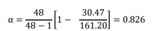
These results indicate that the items have high covariance’s and they measure the same underlying concept hence the questionnaire is reliable for use in the main study.

3.5. Data Analysis

Frequency analysis, relevance analysis, link analysis and severity analysis were used for feature extraction. The frequency analysis identified a pattern in a collection of alerts by counting the number of raw alerts that share some common features such as destination IP address to find the most frequent hit target. The connection between entities were analyzed using the link analysis to
show how two IP addresses are related to each other in a collection of alerts and how IP addresses are connected to the alert types. The association analysis helped in finding the frequent co-occurrences of the values belonging to different attributes. Through association, we traced where many attacks were originating from (source IP) to the target (destination IP and destination Port) and the country of origin.

4. THE PROPOSED METRICS

4.1. Identification of Measurement Attributes
The proposed metrics are extensions of existing security and other network metrics. These metrics include the device value (DV), alert severity (AS) and the alert risk assessment (ARA).
They are intended to measure the following attributes:
i. Device value within the environment
ii. Risk assessment of the alert
iii. Severity of the alert
The metrics identified to measure each of the attributes are;

4.2. Metrics Definition

4.2.1. Device value metric (DV)

The Device Value (DV) metric is an extension of [9]. It is computed as follows

DV=Probability of an alert occurring multiplied by alert weight (base score * environmental score * temporal score) / weight of the alert (base score * temporal score * environmental).

The base score is defined as the importance of the systems account based on the access vector, access complexity, authentication, confidentiality impact, integrity impact and availability impact. Access vector defines how the vulnerability is exploited. It can be local access, adjacent network or network access. The access complexity measures the simplicity of the attack to exploit vulnerability once it has gained access into the system. The complexity can be high, medium or low. The authentication refers to the number of steps an attacker must go through to be authenticated by the target before exploiting vulnerability. It can be multiple authentications, single or none. Confidentiality impact quantifies the sensitivity on confidentiality upon a successful exploited vulnerability, integrity impact quantifies the sensitivity on integrity upon a successful exploited vulnerability and availability impact quantifies the sensitivity on availability of a successful exploited vulnerability. The impact can be complete, partial or none

The environmental scores are user defined. They describe loss of physical asset by damage or theft of property or equipment. They represent the characteristics of vulnerabilities that are associated with user’s IT environment.

The temporal score describes the existence of software update by software developers and easy to use exploit codes by enemies which increase the number of potential attackers including the unskilled and also the level of technical knowledge available to would be attackers. Temporal score focuses on the exploitability, report confidence and the remediation level. Exploitability is the availability of an exploit code to the public that can be used by the potential hackers. Report confidence is the degree of technical knowledge. The would be hackers have about the existence of a vulnerability and remediation level is the existence of workarounds and hot fixes that can provide a solution to the vulnerability before software upgrades are done. The formula to calculate the device value in each server in relation to a particular attack is calculated as shown below

Where n is the first value of i and i is the list of summing up. The equation is simplified as shown below.

Device value indicates the severity level of the target host in relation to an alert. One of the alerts we considered in this paper for computing DV was cross-site scripting referred to as XSS. Its web security vulnerability and works by injecting malicious scripts in a web-based application. When the code executes on the users’ browser, the attacker is able to compromise the application. Its behaviour was observed on mail server, Koha server and ERP server. Based on the CVSS and data collected from the questionnaire, an alert score was computed for each of the servers. Base, temporal and environmental scores for the mail server, Koha and ERP were computed and the results presented in Tables 1, 2 and 3.

i. BaseScore = round_to_1_decimal(((0.6 ∗ Impact) + (0.4 ∗ Exploitability) − 1.5) ∗
𝑓(Impact))
Impact = 10.41 ∗ (1 − (1 − ConfImpact) ∗ (1 − IntegImpact) ∗ (1 − AvailImpact))
Exploitability =20* AccessVector*Access Complexity*Authentication
F (impact) = 0 if Impact = 0, 1.176 otherwise.
ii. TemporalScore = (BaseScore ∗ Exploitability ∗ RemediationLevel ∗
ReportConfidence)
iii. EnvironmentalScore = ((AdjustedTemporal + (10 − AdjustedTemporal) ∗
CollateralDamagePotential) ∗ TargetDistribution)
AdjustedTemporal =TemporalScore recomputed with the Base Score’s Impact
Sub equation replaced with the Adjusted Impact equation.

Table 1. . Base metric group scoring for cross-site scripting on Mail, Koha and ERP servers based on CVSS database and questionnaire score guide

Table 2. Temporal metric group scoring for cross-site scripting on Mail, Koha and ERP servers based on CVSS database and questionnaire score guide

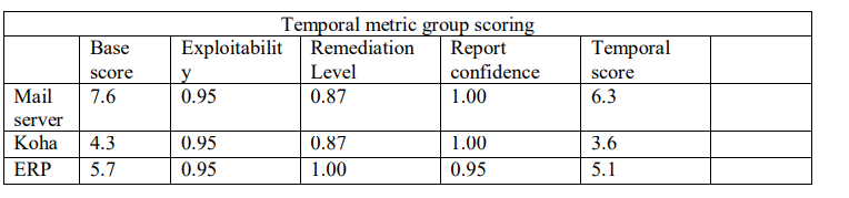
Table 3. Environmental metric group scoring for cross-site scripting on Mail, Koha and ERP servers based on CVSS database and questionnaire score guide

The values on Tables 1, 2 and 3 were used to compute the base, temporal and environmental scores. A summary is shown in Table 4. The next step is to compute the DV of alerts using equation 1. To achieve this, we first compute the alert risk assessment using equation 2.

Table 4. Summary of metric values for Base, temporal and environmental score based on cross-site scripting alert

4.2.2. Alert Risk Assessment Metric

The second stage in working out the device value was to calculate the risk of the alert. In this paper, we adopted the risk assessment formula by [10] whose model was also based on alert risk assessment.

𝑅𝑖𝑠𝑘𝑎𝑠𝑠𝑒𝑠𝑠𝑚𝑒𝑛𝑡 (𝑅𝐴) =  P ∗ D ∗ R  /X  𝐸𝑞𝑢𝑎𝑡𝑖𝑜𝑛 … … … … … .2

Where P is the priority of the alert, D is the device weight and R is the reliability. The risk must not exceed 10. Therefore, X value is obtained by computing the risk using the maximum value of each parameter

𝑅𝐴 = (5 ∗ 5 ∗ 10)/𝑋  = 10               

     𝑋 = 25

𝑇ℎ𝑒𝑟𝑒𝑓𝑜𝑟𝑒 𝑅𝐴 = 𝑃 ∗ 𝐷 ∗ 𝑅/25                                 

Where maximum alert priority is 5, maximum device weight is 5 and alert reliability is 10. The probability of the alerts occurring was also computed as follows:

A number of cross site scripting alert originating from one particular source address within a given time interval was 27 out of a total number of 36.Therefore 27/36 =0.75. The probability of the alert in the range 0 to 1 was 0.75. This probability was used to compute the Pw in Table 5.

Table 5. ARA for cross site scripting alert on servers

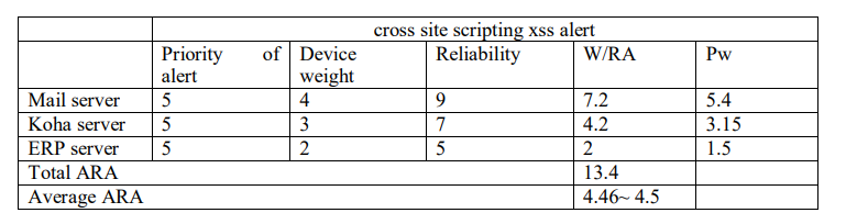
Therefore the DV of mail server, Koha and ERP based on cross site scripting alert is computed as presented below. The values are also shown in Table 6.

𝑤 = 𝑃 ∗ 𝐷 ∗ 𝑅/  25

𝑝𝑤′ = 𝑤(𝑎) ∗ a

Where w or (RA) is the weight of an alert
Pw’ is the weight of an alert multiplied by the probability of an alert occurrence.
a is the probability of an alert occurrence

mail server alert score =pw′ (7.6 ∗ 6.3 ∗ 8.1)/ w(7.6 ∗ 6.3 ∗ 8.1)

Koha server alert score = pw′ (4.3 ∗ 3.6 ∗ 6.8)/ w(4.3 ∗ 3.6 ∗ 6.8)

ERP server alert score =w′ (5.7 ∗ 5.1 ∗ 5)/ w(5.7 ∗ 5.1 ∗ 5)

Total DV = 0.75 + 0.75 + 0.76 = 2.26          

Table 6. DV of Mail server, Koha and ERP server based on cross-site scripting alert

4.2.3. Frequency

Frequency was a metric that was used in alert prioritization. To get the metric value of the alert we compute the total number of times the event occurred divided by the length of time. The equation of the metric is as shown below.

f =a/tt … … … … … … … … … . Equation 3

f is the frequency, tt is the total length of time and a is the total number of similar alerts. In our study we have a total number of 5 similar alerts which occurred within a span of 13 minutes. Frequency can be calculated by dividing the total number of alerts by the total length of time when the alerts occurred. This was done as shown in the working below.

frequency =5/13 = 0.38 alerts per minute

4.2.4. Severity Level Metric

Severity level was the third defined metric that was used in alert prioritization. To get the metric score of the alert we computed as follows:

𝑠𝑒𝑣𝑒𝑟𝑖𝑡𝑦𝑙𝑒𝑣𝑒𝑙 =∑ pw′(bs ∗ rc ∗ rl)/n i=1∑ w(bs) … … … … …… . . Equation 4

Where bs is the base score, rc is the report confidence, rl is the remediation level, pw’ is the probabilistic weight and w is the weight. The alert was confirmed with an official fix. The severity level is computed as follows: base score 7.6, report confidence 1.0, remediation level 0.87. The number of alerts that were generated in a certain alert class within a given period of time was 27 from a total of 36 alerts. A summary of Values for computing severity score are as shown in Table 7.

𝑝𝑟𝑜𝑏𝑎𝑏𝑖𝑙𝑖𝑡𝑦𝑜𝑓𝑎𝑙𝑒𝑟𝑡ℎ𝑎𝑝𝑝𝑒𝑛𝑖𝑛𝑔 =27/36 = 0.75

𝑤(𝑎) =𝑝 ∗ 𝑑 ∗ 𝑟/25

𝑝𝑤′ = 𝑤(𝑎) ∗ 𝑎

Table 7. Summary of metric and weight values for computing the severity score

The Metric values and weight values were used to compute the severity score for the alerts on the three servers as shown in Table 8.

The severity level of the Mail server is:

Table 8. Severity score

5. THEORETICAL VALIDATION RESULTS

All new metrics require to be validated to prove their suitability for their intended use. This burden of prove is granted through a comprehensive, scientific, and objective method of software metrics validation [11]. To certify that a metric is fit and satisfactory for its intended use there must be a prescribed system of regulations for the merits of a metric. This system of warranting the worth of a metric is known as software metrics validation otherwise the software engineering community will find itself filled with metrics that do not conform to the software engineering regulations. Another reason for validation is to verify the efficacy of the attribute measured by the suggested metric[12].Weyuker’s properties have been used to validate complexity metrics by many researchers [14][15][16][17][18][13]. These properties are used to assess the precision of measure and in turn lead to the definition of good notions of software complexity. With the help of these properties, one can determine the most suitable measure among different available complexity measures [19]. A good complexity measure should satisfy Weyuker’s properties [20]. Therefore, the proposed metric have been validated using weyuker’s properties and Kaner’s framework.

5.1. Validation with Weyuker’s Properties

Property 1: (∃P)(∃Q)(|P|≠|Q|) where P and Q are the two different alerts.

This property states that a measure should not rank all metric as equally complex. A good metric must have the capability to distinguish between the impacts of two different attack alerts on different programs and return different measurement.

All the metrics proposed DV, ARA, and AS return different complexity value for any two alerts that are not identical therefore they all satisfied property 1

Property 2: Let c be a non-negative number, and then there are finitely many different attack alerts impact of complexity c.

This property asserts that if an alert changes then the complexity value changes. DV, ARA and AS can detect change in complexity when the attack types is varied, Therefore all the proposed metrics satisfied weyuker’s property 2.

Property 3: There can exist distinct alerts P and Q such that |P|=|Q|. This property asserts that there exist two different alerts whose impact is identical. For example two alerts could differ in naming, source, and in type but may otherwise define the variables with the same data type and value. Two alerts P and Q will have the same complexity provided they are identical in terms of impact and exploitability.

Property 4: (∃P)(∃Q)(P=Q & |P|≠|Q|)

There can be two alerts P and Q whose external features look the same however due to different internal structure |p| is not equal to |Q|. This property asserts that two alerts could look identical externally but be different in their internal structure. Two alerts could be from the same source but be different in type and impact. A viable metric should have the capacity to analyse beyond the external characteristics and differentiate metrics formed on their internal structure. Therefore all the proposed metrics satisfied this property.

Property 5: (∀P) (∀Q) (⎢P ⎢≤⎢P; Q ⎢&⎮Q ⎮≤⎢P; Q⎮).

This property declares that if we combined two alerts impacts P and Q the new metric value must be greater than or equal to the value of the individual alert impact. All the proposed metric return numeric values meaning they satisfy this property.

Property 6: (∃P)(∃Q)(∃R)(⎮P⎮=⎢Q⎮)&⎮P;R⎮≠⎢Q; R⎮).

This property states that if a new alert is appended to two alerts which have the same alert impact complexity, the alert impact complexities of two new combined alert are different or the interaction between P and R can be different than interaction involving Q and R thus leading to different complexity values for P+ R and Q + R. The metrics DV, ARA, and AS assign fixed value to each of their alerts, Due to these fixed values every time two alerts are combined they return different values hence they failed to satisfy this property.

Property 7: If you have two alerts P and Q which have the same number of attributes in a permuted order then (⎮P ⎮≠⎢Q⎮).

This property states that permutation of attributes within the item being measured can change the metric values. Therefore, if two alerts which have same number of similar attribute but differ in their ordering, then their metric values are not the same. In the case where alerts values are fixed in relation to their impact and you only change the permutation of the order of values then all the proposed metrics will return the same level of complexity. Hence the metrics proposed did not satisfy this property.

Property 8: If P is renaming of Q, then ⎮P ⎮= ⎢Q⎮.

When alert name change it will not affect the complexity of the alert. Even if the attributes name in the alert change, the alert complexity should remain unchanged. The metric values for all the proposed metrics are value measures, risk weight measures, or impact measures and they all return numeric values. Therefore all the proposed metrics satisfies this property.

Property 9: (∃P) (∃Q) (⎮P ⎮+ ⎢Q⎮). < (⎮P; Q⎮).

This property states that the alert impact complexity of a new alert impact combined from two alerts impacts is greater than the sum of two individual alert impact complexities. In other words, when two alert impacts are combined, they can increase the complexity metric value. The growth in alert complexity happens when new alert attributes are added or when a new node is added and none of the node has negative value meaning that the new metric value is equal to or greater than the sum of the two individual alert impact complexities. All metrics DV, ARA and AS satisfied this property.

5.2. Validation with Kaner’s Framework

In this study, we evaluate our metrics using ten questions according to [20][12].

i.What is the purpose of this measure?
The purpose of the measure is to evaluate the complexity and severity of the alerts so that we can inform network security team.
ii. What is the scope of this measure?
The proposed metric will be used by network security team to enhance the security of their network systems.
iii. What attribute are we trying to measure?
The attributes to be measured will be severity, importance, and weight.
iv. What is the normal dimension of the attribute we are trying to measure?
The importance of devices will be measured through the impact of alerts from attackers. Other measurement will be severity and risk of alerts all of which can be measured on an
ordinal scale.
v. What is the natural variability of the attribute?

The impact of the alerts will be ranked by network security experts who’s their opinions can vary based on experience and environment they are subjected to.
vi. What is the metric (the function that assigns a value to the attribute)? What measuring
instrument do we use to perform the measurement?
The proposed metrics have been computed statistically using a developed metric tool and measured using fuzzy logic.
vii. What is the normal scale for this metric?
The natural scale for all proposed metrics falls under interval scale.
viii. What is the natural variability of readings from this instrument?
There will be no measurement error since the measurement will be done using a software tool that will be tested to ensure it is free from bugs.
ix. What is the relationship of the attribute to the metric value?
The base score, temporal and environmental score are directly related to the proposed metric therefore we can measure the device value, severity and the risk level using the proposed metric.
x. What are the natural and foreseeable side effects of using this instrument?
The tool is tested and functioning very well with no negative effect unless brought by new advancement in technology.

EXPERIMENTAL RESULTS

6.1. Experiment Environment

A Proxmox virtual environment was set up to host Modern Honey Net (MHN) server, snort, firewall, dionaea and cowrie virtual machines. Proxmox VE is complete open source server platforms for enterprise virtualization which help cut costs for IT departments and add server stability and efficiency. To install Proxmox Virtual Environment; we downloaded Proxmox ISO Image, prepared the Installation Medium, Launched the installer and ran Proxmox. Second VMs were created by uploading an ISO image which contained ubuntu-18.04-server to Proxmox VE. The VMs were created in Proxmox VE where the hard disk storage space, the number of cores and the RAM size of the VMs were defined. Lastly the OS was installed in the virtual machines. The experiment was carried out for two weeks in a controlled environment. All the alerts from the sensors were collected in the MHN server. Figure 1 shows a virtualised MHN server.

Figure 1. MHN server

6.2. Payloads and Attacks Report

Various sensors were deployed as illustrated in Appendix 1. Snort was able to capture 27180 alerts, cowrie 0, and dionaea 96824 alerts within a period of one week. The output from the payload report indicated the source IP, destination port, the signature, the classification and reporting sensor as shown in Figure 2.

Figure 2. Payload report

The output from the attack report indicated the source IP, destination port, the protocol, the sensors, date and time of attack and the country of origin as shown in Figure 3.The alerts collected were mapped on a vulnerability database in relation to the response from the questionnaire. The device value, severity level of the alert, frequency and weights were computed based on the metrics tool. 

Figure 3. Attacks report

6.3. Metrics Values

A metrics tool developed for the study was used to compute the alert score based on device value, weight of an alert, frequency of the alert and the severity level of the alert The device value metric for alert A2 at 1.13 is lower than the metric value for alert 1though they have the same number of attributes. This is true because the weight and frequency score of alertsA2 is lower than alert A1.The goal of this metric is to show the criticality of the target server machines. The criticality of these machines depends on the operating system, applications and services running on them. The severity score metric for alert A2 at 0.65 is higher than all
others because its base score is high. The metric measures the impact level posed by a particular alert. Alert A1 has the highest weight of 5 because of its high priority, value and relevance. The output of device value, severity score, frequency and weight are subjected to fuzzy rules to obtain output values for each individual rule. These outputs are weighted and averaged in order to have
one single output that is defuzzified into a crisp value. This is the alert relevance that represents alert impact on the server machines. This is shown in Table 10.

Table 10. Metricscores of alerts

6.4. Fuzzifying the Metrics

Results from the device value, alert severity, frequency and alert risk assessment metrics serve as the inputs to the fuzzy logic inference engine. These values are subjected to the fuzzy rules to obtain output values for each rule. An average of these values is computed to form one single output value. The output value is then defuzzified to map the output of the inference engine into
a crisp value

Fuzzy logic is composed of the rule based, fuzzification, inference engine and the defuzzification. The rule based contains a set of rules that govern decision making. They decide the output based on the inputs. The fuzzification is used to change the inputs into fuzzy sets. The inference engine compares the input fuzzy with the rules and chooses rules to be fired. Defuzzification converts the output of the inference engine into crisp values as shown in Figure 4

Figure 4. Rule Viewer with the Relevance Result

The rule viewer displays the output of the entire fuzzy inference process and shows how the membership function influences the output. Figure 4 shows the input as 1.66, 0.55, 0.38, and 5 which were fuzzified and gave the output of 8.5. This meant the alert relevance was medium and qualified to be sent to the next component for alert correlation. However the alert is discarded if it is of low relevance as shown in Figure 5.

Figure 5. Rule Viewer with the Relevance Result

Figure 5 shows the input as 1.5, 0.45, 0.31, and 4.1 which were fuzzified and gave the output of 2.83. This meant the alert relevance was low hence needed to be discarded since it did not qualify to be taken to the next component for alert correlation.

6.5. Validation of the Proposed Model

Validation is a vital process in any research as it affirms that the results obtained in a study are valid and consistent[21]. Therefore, before discussing the results, validation of the model was done using the Analytical Hierarchical Process (AHP) framework to ascertain that the tool is giving valid results.

The validation process of AHP followed the three stages methodology [22]. First development of the hierarchical structure for alert relevance prediction as the goal at the top level, the device value, severity and alert risk assessment and frequency as attributes/ criteria in the second level and the alternatives represented by the alerts at the third level. Figure 6 shows the AHP Hierarchical structure for alert relevance prediction in this research.

Figure 6. AHP Hierarchical Structure for Alert Relevance Prediction

The second was creation of a pair wise comparison matrix. At each level of the hierarchy, the relationships between the elements are established by comparing the elements in pairs. A pair wise comparison was done by forming a matrix to set priorities. The comparison starts from the top of the hierarchy to select the criterion, and then each pair of elements in the level below is compared. These judgements are then transformed to the scale of 1 to 9 that represent the relative importance of one element over the other with respect to the property. The scale of 1 to 9 has the following qualitative meaning.1 for equal importance, 3 moderate importance, 5 strong importance, 7 very strong importance, 9 extremely importance with 2,4,6,8 as intermediate values and 1/3, 1/5, 1/7, 1/9 as values for inverse comparison.

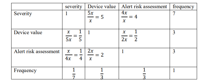
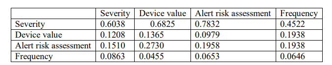
The values in the pair-wise matrix depend on the type of alert used when modelling the model being validated. This proof was obtained from the international vulnerability database. For example, if the alert was a Web application attack ,then device value was of strong importance than severity, ARA was of moderate to strong importance than severity, Alert Risk Assessment is of equal to moderate importance than device value Therefore, relating these judgments to the Saaty scale lead to formation of expression such that: If device value = x value then Alert Risk Assessment = 2x value and if severity = x value then device value = 5x value and if severity = x value Alert Risk Assessment = 4x value. The first step is to generate a pairwise comparison matrix as shown in Table 11.

Table 11.Pair-wise Comparison Matrix

The sum of each column is calculated by first converting the fractions to decimals to get a non normalised pair-wise comparison matrix. This is shown in Table 12.

Table 12.Non normalised Pair-wise Comparison Matrix

The next step is to generate a pair-wise normalised matrix by dividing each value of a column by the total which is the normalization factor. The above arithmetic operations indicate that normalization is applied to rescale the priorities of the criteria and use them to weight the priorities of the alternatives before they are normalized[22]. The calculations in Table 13 are as
show Figure 7.

Figure 7.computation of a Normalised pair-wise comparison matrix

Table 13. Normalised pair-wise comparison matrix

The next step is to compute the criteria weight in Table 14 by summing all the values in each row and dividing the total by the number of criteria. The formula is as shown below.

= 𝑠𝑢𝑚 𝑜𝑓 𝑎𝑙𝑙 𝑡ℎ𝑒 𝑐𝑟𝑖𝑡𝑒𝑟𝑖𝑎 𝑖𝑛 𝑒𝑎𝑐ℎ 𝑟𝑜w/𝑛𝑢𝑚𝑏𝑒𝑟 𝑜𝑓 𝑐𝑟𝑖𝑡𝑒𝑟𝑖𝑎 

First row:0.6289 + 0.6002 + 0.6861 + 0.5000/4= 0.6038

Second row:0.1258 + 0.1200 + 0.0858 + 0.2143/4= 0.1365

Third row:0.1572 + 0.2401 + 0.1715 + 0.2143/4= 0.1958

Fourth row:0.0898 + 0.0400 + 0.0572 + 0.0714/4= 0.0646

Table 14. Normalised pair-wise comparison matrix with criteria

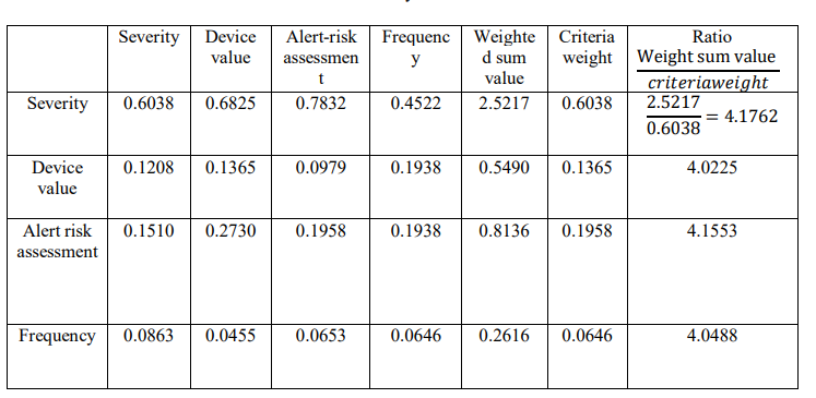
Third was calculating the Consistency ratio in Figure 8 to check whether the calculated values were correct or not as shown in Table 15. In this step the pair-wise matrix which is not normalised is taken and each value in the column multiplied by criteria value. This is computed as shown below:

Figure 8. computation of Consistency ratio

Table 15. Consistency matrix

The next step is computing the weighted sum value by adding the row elements of the consistency matrix as shown in Table 16.

Table 16. Consistency matrix with weighted sum value

The ratios of weighted sum value and criteria weights are computed for each row in Table 17.

Table 17.Consistency Matrix with Ratios

These ratios are then used to compute the maximum Lambda which is computed by getting the average of the ratios as shown in the working below.

𝜆 𝑚𝑎𝑥 =𝑠𝑢𝑚 𝑜𝑓 𝑎𝑙𝑙 𝑒𝑙𝑒𝑚𝑒𝑛𝑡𝑠 𝑖𝑛 𝑡ℎ𝑒 𝑟𝑎𝑡𝑖𝑜 𝑐𝑜𝑙𝑢𝑚n/4

𝜆 𝑚𝑎𝑥 = 4.1007

The 𝜆𝑚𝑎𝑥 obtained was used to compute consistency index given by the formula:

Consistency index =𝜆 𝑚𝑎𝑥 − 𝑛 /n − 1

CI =4.1007 − 1/4-1

=0.03358

Finally the consistency ratio (CR) was computed by dividing the consistency index by random index. CR is a standard used to affirm whether the matrix is reasonably consistence and the model is giving valid predictions. The random index is the consistency index of randomly generated pair wise matrix of size n[23].In this study the random index for n equal to 4 is 0.90.

Therefore consistency ratio=𝐶I/RI

Consistency ratio =0.03358 /0.90

CR is 0.037311

On a scale from O-1, inconsistency should not exceed 0.10.Thus, CR < 0.1, the matrix can be acceptable as consistent matrix, contrarily CR ≥ 0.1, the matrix should be modified until an acceptable one. In our study our CR is0.037311< 0.10which is the standard. Therefore it implies that the matrix is reasonably consistence. This indicates that the decisions made by the model are
reliable and the decision-maker gives consistent results.

7. DISCUSSION

Device importance, alert impact and alert risk were validated using weyuker’s properties. Findings show that DV, AS and ARA failed to satisfy weyuker’s property 6 and 7. This is because each alert is assigned fixed value which prevents them from detecting extra environmental impact that could arise from the same alert. Also, since alert values are fixed changing the permutation of the order of values does not affect the level of complexity.

Kaner’s framework[24] was also adopted and used to gauge the practicality, consistency and correlation of the defined metrics. This framework formed part of theoretical validation and enhanced the construct validity of experiments. it was observed that Correlation existed among the attributes of the proposed metric . A change in one attribute proportionally affected the other attributes outcome. This implied that the proposed metrics were Consistent and linearly related.

The researcher further used Kaner framework to confirm the practicality of the metrics. This framework required a response to its 11 questions, and all the questions were responded to positively demonstrating quality and ability of metrics to capture what they were supposed to measure and is a proof that they can be applied to a real-life scenario.

From the experiment results the device value metric for alert A1 at 1.66 was higher than its severity score of 0.55. This is reasonable because device value metric has more attributes than severity metric. The frequency score for alert A1 at 0.38 is higher than all other which make sense because it has higher number of recurrence in a given time interval than other alerts. The final metric weight, is highest in alert A1 at 5, this is reasonable because its priority and relevance are more weighty as compared to other alerts.

Metric values for each alert were computed and fuzzified to give alert relevance which was subsequently assigned to their respective alerts classifications. These classifications were low level, medium level and high level alert relevance classification. Every alert belonged to one of the three classifications. After fuzzification the alerts relevance for alert A1 is the highest at 8.5.
This means it has the highest weight/ impact to the systems.

8. CONCLUSIONS AND FUTURE WORK

From the experiment, we observed that a lot of repetitive alerts were generated that increased the network communication and the alert processing load. The system admin was overwhelmed with the alert analysis pressure which took a lot of time. We have presented an approach to manage unnecessary alerts generated by multiple IDS products. The critical modules of the approach are
Alert Scoring and fuzzy logic modules. The Alert Scoring module uses metrics scores to improve the quality of the raw alerts from multiple sensors by filtering out those with low scores. We defined three metrics related to Device value, Risk assessment and Severity of the alert which were fuzzified to get alert relevance. In the experiment dataset collected from different sensors was used to offer a more comprehensive solution to detect new attacks that are not detected by IDS alone. The fuzzy logic modules received results from the metric as input to the fuzzy logic inference engine to investigate its impact and assign a single score to each alert. A simulation was conducted to demonstrate the applicability of metrics in alert scoring.

In future, we plan to use the results obtained from this study to design a novel alert correlation model that will help to filter the unnecessary attacks (low level impact) and classify similar alerts together to reduce alert analysis time. We also plan to integrate AI techniques and algorithms,

particularly those that handle the representation of logic as well as reduction in the size of the database (alerts) in order to improve the alert management process, hence improving aggregation process and reducing unnecessary alerts.

REFERENCES

[1] L. M. L. de Campos, R. C. L. de Oliveira, and M. Roisenberg, “Network Intrusion Detection System Using Data Mining,” pp. 104–113, 2012, doi: 10.1007/978-3-642-32909-8_11.
[2] M. M. S.Vijayarani & Sylviaa.S, “INTRUSION DETECTION SYSTEM – A,” Int. J. Secur. Priv. Trust Manag., vol. 4, no. 1, pp. 31–44, 2015.
[3] D. Hutchison, Advances in Information, no. November. 2013. doi: 10.1007/978-3-030-26834-3.
[4] S. Salah, G. Maciá-fernández, and J. E. Díaz-verdejo, “A model-based survey of alert correlation techniques,” Comput. Networks, vol. 57, no. 5, pp. 1289–1317, 2013, doi: 10.1016/j.comnet.2012.10.022.
[5] H. A. Khan et al., “IDEA: Intrusion Detection through Electromagnetic-Signal Analysis for Critical Embedded and Cyber-Physical Systems,” IEEE Trans. Dependable Secur. Comput., vol. 18, no. 3, pp. 1150–1163, 2021, doi: 10.1109/TDSC.2019.2932736.
[6] G. Dogan and T. Brown, “ProTru: A Provenance Based Trust Architecture for Wireless Sensor Networks,” Int. J. Netw. Manag., pp. 17–31, 2014, doi: 10.1002/nem.
[7] R. Xi, X. Yun, Z. Hao, and Y. Zhang, “Quantitative threat situation assessment based on alert veri fi cation,” no. March, pp. 2135–2142, 2016, doi: 10.1002/sec.
[8] G. Dogan and T. Brown, “ProTru: A Provenance Based Trust Architecture for Wireless Sensor Networks,” Int. J. Netw. Manag., no. March, pp. 17–31, 2014, doi: 10.1002/nem.
[9] K. Alsubhi, I. Aib, and R. Boutaba, “FuzMet : a fuzzy-logic based alert prioritization engine for intrusion detection systems,” 2011, doi: 10.1002/nem.
[10] E. M. Chakir, M. Moughit, and Y. I. Khamlichi, “An Effecient Method for Evaluating Alerts of Intrusion Detection Systems National School of Applied Sciences USMBA,” 2017.
[11] M. Alharthi and W. Aljedaibi, “Theoretical Validation of Inheritance Metric in QMOOD against Weyuker ’ s Properties,” vol. 21, no. 7, pp. 284–296, 2021.
[12] G. M. Muketha, A. A. A. Ghani, and R. Atan, “Validating structural metrics for BPEL process models,” J. Web Eng., vol. 19, no. 5–6, pp. 707–723, 2020, doi: 10.13052/jwe1540-9589.19566.
[13] G. M. Muketha, A. A. A. Ghani, M. H. Selamat, and R. Atan, “Complexity metrics for executable business processes,” Inf. Technol. J., vol. 9, no. 7, pp. 1317–1326, 2010, doi: 10.3923/itj.2010.1317.1326.
[14] K. Maheswaran and A. Aloysius, “Cognitive Weighted Inherited Class Complexity Metric,” Procedia Comput. Sci., vol. 125, pp. 297–304, 2018, doi: 10.1016/j.procs.2017.12.040.
[15] A. K. Jakhar and K. Rajnish, “Measuring Complexity, Development Time and Understandability of a Program: A Cognitive Approach,” Int. J. Inf. Technol. Comput. Sci., vol. 6, no. 12, pp. 53–60, 2014, doi: 10.5815/ijitcs.2014.12.07.
[16] D. Beyer and P. Häring, “A formal evaluation of dep degree based on Weyuker’s properties,” 22nd Int. Conf. Progr. Comprehension, ICPC 2014 – Proc., pp. 258–261, 2014, doi: 10.1145/2597008.2597794.
[17] K. Rim and Y. Choe, “Software Cognitive Complexity Measure Based on Scope of Variables,” CoRR, vol. abs/1409.4, 2014.
[18] P. Gandhi and P. K. Bhatia, “Analytical Analysis of Generic Reusability : Weyuker ’ s Properties,” vol. 9, no. 2, pp. 424–427, 2012.
[19] M. Aggarwal, V. K. Verma, and H. V. Mishra, “An Analytical Study of Object-Oriented Metrics (A Survey),” Int. J. Eng. Trends Technol., vol. 6, no. 2, pp. 76–82, 2013, [Online]. Available: http://www.ijettjournal.org
[20] J. G. Ndia, G. M. Muketha, and K. K. Omieno, “a Survey of Cascading Style Sheets Complexity Metrics,” Int. J. Softw. Eng. Appl., vol. 10, no. 03, pp. 21–33, 2019, doi: 10.5121/ijsea.2019.10303.
[21] N. Saardchom, “The validation of analytic hierarchy process (AHP) scoring model,” Int. J. Liabil. Sci. Enq., vol. 5, no. 2, p. 163, 2012, doi: 10.1504/ijlse.2012.048472.
[22] R. W. Saaty, “The analytic hierarchy process-what it is and how it is used,” Math. Model., vol. 9, no. 3–5, pp. 161–176, 1987, doi: 10.1016/0270-0255(87)90473-8.
[23] M. Brunneli, Introduction to the Analytic Hierarchy Process. 2015.

[24] C. Kaner and W. P. Bond, “Software Engineering Metrics : What Do They Measure and How Do We Know ?,” 10Th Int. Softw. Metrics Symp. Metrics 2004, vol. 8, pp. 1–12, 2004, [Online]. Available: http://testingeducation.org/a/metrics2004.pdf

Appendix 1: Sensors

The network monitoring sensors automatically collects logs and stores them in a central location. These logs contain valuable network threat information about attack source, protocols used, date and time of attack and countries of origin that can be extracted to provide a perspective of your network’s overall security standing.